Combining two fundamental paradigms to learn more from biological experiments
Biological experiments typically yield observations that clearly suggest non-linear relationships between the measured variables and, often, are laborious and afford a limited number of observations and repetitions. Systems of ordinary differential equations offer a way to build mechanistic models of, complex, non-linear phenomena. Bayesian inference offers a paradigm to embrace the uncertainty of real-world experiments and exploit our prior knowledge. Biology is complex, experiments are difficult, but we do have a few successful modeling paradigms, there are also clear physical constraints to what biological systems can do, and a rich literature of quantitative experiments. In this post, I show and example of how Bayesian Data Analysis and systems of differential equations can be combined to learn the most we can from a single experiment with a few measurements. All the code used in this post and be found here.
A toy model of a growing yeast culture
The toy model below was built to simulate a simple experiment. Imagine you procure a few grams of dry yeast and want to estimate its viability. That is, what fraction of the dry yeast weight is composed of living yeast cells?
One experiment you could try, would be to inoculate 1 gram of dry yeast in a 1 liter batch fermentation and measure the glucose and biomass concentrations at a few time points. What could you learn about the yeast you bought through such an experiment?
Let’s begin by making a toy model to simulate the experiment. Here I present a simple model of a yeast culture. It consists of two dynamic mass balances, one for biomass and one for glucose. Notice that the two balances differ only in the sign of the expression and in the division by Yxs in the glucose balance. In a world without noise or uncertainty, we could infer all the parameters in the system by measuring either glucose or biomass. In the real world there is uncertainty, and the measurement of some variables is more trustworthy than others. We thus benefit from performing redundant measurements. Here is the system of Ordinary Differential Equations for our toy example:
Where glc stands for glucose in mmol, X stands for biomass dry weight in g, μ is the maximum growth rate, Yxs is the biomass yield in mmol glucose per gram biomass, and f(glc) is a kinetic expression that determines the rate at which glucose can be consumed. It is described by the following rate law:

Parameters and initial conditions
The model parameters are based on measurements taken from bakers yeast growing aerobically on sugar.

The initial glucose amount is known to us (we prepared the medium) to be 100 mmol. The initial biomass, the viability of the dry yeast, is unknown, we want to infer it. For the simulation generating the synthetic experimental data we will use an initial biomass amount of 0.2 grams.
Simulating the experiment
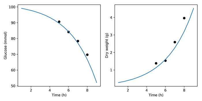
The figure above shows the output of simulating our toy model in blue. The black circles at 5, 6, 7 and 8 hours represent the observations we made during this experiment. They were calculated by adding noise to simulation results at those times. Below we will imagine that all we know about our yeast is that it generated those eight observations (four time points and two variables), when we inoculated 1 gram dry weight in a medium with 100 mmol glucose.
Bayesian Data Analysis
Choosing prior probability distributions
There are two parameters to infer, the biomass yield on glucose, the maximum specific rate of glucose consumption; and two initial conditions.
Biomass yield on glucose
The maximum possible biomass yield on glucose is given by the hypothetical situation in which all the consumed glucose would be incorporated into biomass. That is none of the glucose would be lost in decarboxylating reactions nor catabolized to drive biosynthesis. Assuming the following elemental biomass composition: C₁H₁.₈N₀.₂O₀.₅ and that ammonia is used as nitrogen source, we can write a biomass synthesis reaction:
which implies a maximum biomass yield on glucose (Yxs) of 0.139 grams dry weight per mmol glucose.
Maximum biomass specific growth rate
Before hand we know little about our yeast. We do know that it is a yeast, and that yeast grows slower than Escherichia coli, which in synthetic medium has a reported maximum growth rate of 0.89 1/h [reference].
Initial conditions
We know the initial glucose concentration within experimental error. We expect our solution to be within 1 or 2 mmol of our intended concentration of 100 mmol. But we know much less about the amount of viable cells we inoculate our culture with. We do know that we added 1 gram, and that the fraction of viable cells is larger than zero and smaller than one.
Prior probability distributions
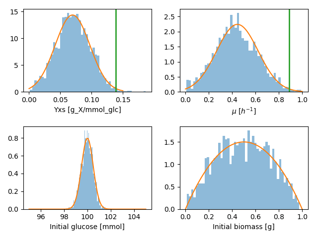
I chose to use normal probability distributions to model all priors. For the two parameters, the mean and standard deviation were chosen so that the maximum values, we calculated above, would be possible but rather unlikely. I modeled the prior for initial glucose as normal distribution with a small standard deviation, and the initial biomass as a symmetric beta distribution.
Estimating posterior probability distributions
Here I used Stan to infer the distribution of parameters compatible with the observations. Stan provides a built-in system to solve ODEs [link]. This is the Stan model code:
functions {
    real[] myodes(
        real t,
        real[] y,
        real[] p,
        real[] x_r,
        int[] x_i
        )
        {
            real dydt[2];
            dydt[1] = -y[2] * (p[1] / p[2]) * (y[1]/1) / (1 + (y[1]/1));
            dydt[2] = (y[2] * p[1] * (y[1]/1) / (1 + (y[1]/1)));
            return dydt;
        }
}data {
    int<lower=1> N;
    int<lower=1> T;
    real y[N, 2];
    real t0;
    real t_obs[N];
    real t_sim[T];
    }transformed data {
    real x_r[0];
    int x_i[0];
}parameters {
    real<lower=0> y0[2]; // init
    vector<lower=0>[2] sigma;
    real<lower=0> p[2];
}transformed parameters {
    real y_hat[N, 2];
    y_hat = integrate_ode_rk45(myodes, y0, t0, t_obs, p, x_r, x_i);
}model {
    sigma ~ normal(0, 1);
    p[1] ~ normal(0.445, 0.178);
    p[2] ~ normal(0.0695, 0.027800000000000002);
    y0[1] ~ normal(100, 0.5);
    y0[2] ~ beta(2, 2);
    for (t in 1:N)
        y[t] ~ normal(y_hat[t], sigma);
}generated quantities {
    real y_hat_n[T, 2];
    real y_hat_sigma[T, 2];y_hat_n = integrate_ode_rk45(myodes, y0, t0, t_sim, p, x_r, x_i);
    // Add error with estimated sigma
    for (i in 1:T) {
        y_hat_sigma[i, 1] = y_hat_n[i, 1] + normal_rng(0, sigma[1]);
        y_hat_sigma[i, 2] = y_hat_n[i, 2] + normal_rng(0, sigma[2]);
        }
}
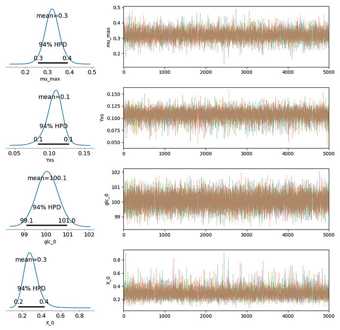
There are several checks to diagnose the representativeness of the posterior samples we obtain in MCMC runs. First, the traceplots of four chains (right-hand-side plots) are well mixed and seem to explore the parameter space without getting stuck in different regions at different iterations. The summary table below, generated by Stan, show that the number of effective samples (n_eff — number of uncorrelated samples) is larger than 5000 for all parameters, and that Gelman-Rubin statistic is 1.0 for all parameters. Also, and as important, the density plots and the High Density Probability (HPD) intervals are almost identical when the model is ran with a different seed.

The HPD intervals divided by their mean show that the initial glucose (y0[1]) is rather certain (we had a certainty in the prior already). Based on the HPD intervals, we’d expect that the mass fraction of dry yeast occupied by viable cells is between 0.17 and o.46. We set out to learn about this fraction, before the experiment and analysis we only knew that the fraction was constrained between 0 and 1. After the observations we narrowed the range to possibilities to 30% of our initial range.
Comparing prior and posterior distributions
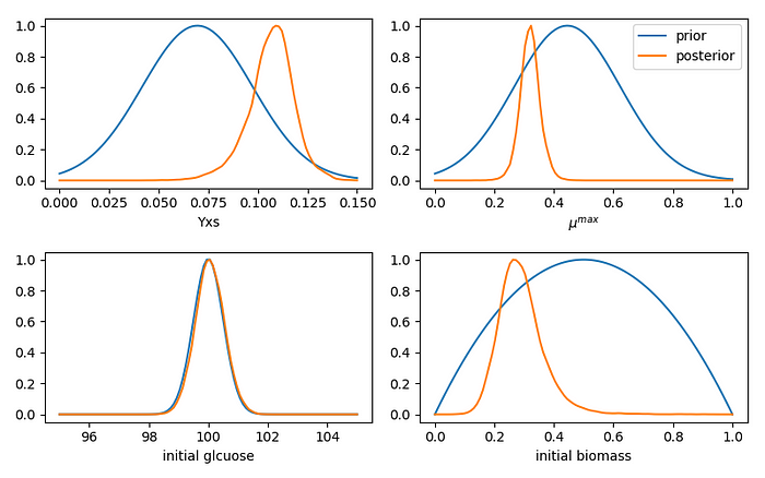
With the exception of initial glucose, the posterior probabilities are more concentrated than their priors. We were very certain about our initial glucose amount, and our observations do not seem to contest that certainty. In the other three cases, the observations enabled us to update our expectations, which moved away from the middle of the range we set up in our priors.
Learning from the posterior
Samples from the posterior probability distribution show a negative correlation between the maximum growth rate (μ) and the initial biomass amount. The posterior also shows a positive, though weaker, correlation between the maximum growth rate and the biomass yield. The figure below encodes the initial biomass and maximum growth rate spatially, while the biomass yield is used to color the dots.
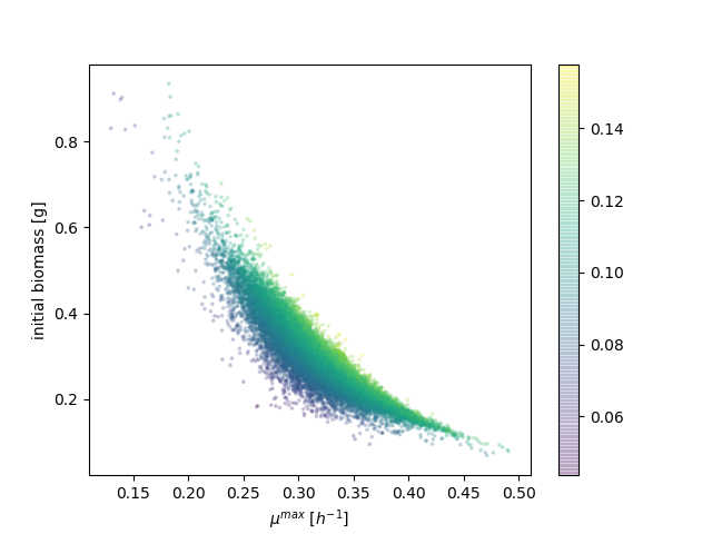
These correlations tell us that, in fitting the observations, a high initial biomass amount can be counterbalanced by a low growth rate, and that a low growth rate can be counterbalanced by a high yield. There is thus a family of model parameters that could explain the observations equally well.
Model predictions
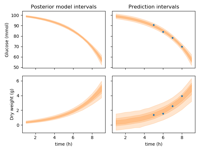
Having obtained representative samples from the posterior probability distribution, one can then forward simulate the model create a posterior distribution of model outputs. If in addition we use the estimated variance of the measurements, we postulate predictions for future, independent, repetitions of the experiment. The plot below shows the 50, 75 and 95% credible intervals for the model outputs (left-hand-side) and independent repetitions of the experiment (right-hand-side). The data points used to fit the model are shown to fall within the 95% credible intervals, suggesting that the data generating model we obtained could have indeed generated those observations.
