Guide to Optimization algorithms for Deep Neural Networks

Optimization is without a doubt in the heart of deep learning. Gradient-descent-based methods have been the established approach to train deep neural networks.

As pertinently described in Wikipedia:

Optimization is the selection of the best element (with regard to some criterion) from some set of available alternatives.

In the simplest case, an optimization problem consists of maximizing or minimizing a real function by systematically choosing input values from within an allowed set and computing the value of the function.

In the case of Machine Learning, optimization refers to the process of minimizing the loss function by systematically updating the network weights. Mathematically this is expressed as w’ = argmin_w{L(w)}w’=argminw​L(w), given a loss function $L$ and weights $w$

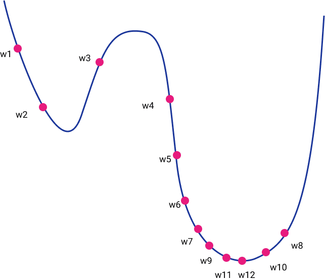
Intuitively, it can be thought of as descending a high-dimensional landscape. If we could project it in 2D plot, the height of the landscape would be the value of the loss function and the horizontal axis would be the values of our weights w. Ultimately, the goal is to reach the bottom of the landscape by iteratively exploring the space around us.

Gradient descent

Gradient descent is based on the basic idea of following the local slope of our landscape. We essentially introduce physics and the law of gravity in the mix. Calculus provides us with an elegant way to calculate the slope of the landscape, which is the derivative of the function at this point (also known as the gradient) with respect to the weights.

Learning rate is a constant value known as learning rate and determines the step size at each iteration while moving toward a minimum of a loss function

Algorithmically this can be expressed in Python as below:

Visually, we can imagine the following diagram which corresponds to a 2d space.

In practice, there are 3 main different variants of gradient descent when it comes to deep learning.

Batch gradient descent

The equation and code presented above actually referred to batch gradient descent. In this variant, we calculate the gradient for the entire dataset on each training step before we update the weights.

You can imagine that since we take the sum of the loss of all individual training examples, our computation becomes quickly very expensive. Therefore it’s impractical for large datasets.

Stochastic gradient descent

Stochastic Gradient Descent (SGD) was introduced to address this exact issue. Instead of calculating the gradient over all training examples and update the weights, SGD updates the weights for each training example {x_i,y_i}xi​,yi​

In python, this can represented as follows:

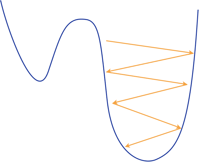
As a result, SGD is much faster and more computationally efficient, but it has noise in the estimation of the gradient. Since it updates the weight frequently, it can lead to big oscillations, which makes the training process highly unstable.

You can imagine that we continuously walk in a zig-zag fashion down the landscape which results in keep overshooting and missing our minimum. Although for the same reason, we can easily get away from local minimums and keep searching for a better one.

Mini-batch Stochastic Gradient Descent

Mini batch SGD sits right in the middle of the two previous ideas combining the best of both worlds. It randomly selects $n$$ training examples, the so-called mini-batch, from the whole dataset and computes the gradients only from them. It essentially tries to approximate Batch Gradient Descent by sampling only a subset of the data. Mathematically:

In practice, mini-batch SGD is the most frequently used variation because it’s both computationally cheap and results in more robust convergence.

Note that in the bibliography the term SGD often refers to mini-batch SGD. So, keep in mind that from now one we will use the same terminology.

Concerns on SGD

However, this basic version of SGD comes with some limitations and problems that might negatively affect the training.

1. If the loss function changes quickly in one direction and slowly in another, it may result in a high oscillation of gradients making the training progress very slow.
2. If the loss function has a local minimum or a saddle point, it is very possible that SGD will be stuck there without being able to “jump out” and proceed in finding a better minimum. This happens because the gradient becomes zero so there is no update in the weight whatsoever.

A saddle point is a point on the surface of the graph of a function where the slopes (derivatives) are all zero but which is not a local maximum of the function

3. The gradients are still noisy because we estimate them based only on a small sample of our dataset. The noisy updates might not correlate well with the true direction of the loss function.
4. Choosing a good loss function is tricky and requires time-consuming experimentation with different hyperparameters.
5. The same learning rate is applied to all of our parameters, which can become problematic for features with different frequencies or significance.

To overcome some of these problems, many improvements have been proposed over the years.

Adding Momentum

One of the basic improvements over SGD comes from adding the notion of momentum. Borrowing the principle of momentum from physics, we enforce SGD to keep moving in the same direction as the previous timesteps. To accomplish this, we introduce two new variables: velocity and friction

• Velocity $v$ is computed as the running mean of gradients up until this point in time and indicates the direction in which the gradient should keep moving towards
• Friction $\rho$ is a constant number that aims to decay

At every time step, we update our velocity by decaying the previous velocity on a factor of $\rho$ and we add the gradient of the weights on the current time. Then we update our weights in the direction of the velocity vector

But what do we gain with momentum?

• We can now escape local minimums or saddle points because we keep moving downwards even though the gradient of the mini-batch might be zero
• Momentum can also help us reduce the oscillation of the gradients because the velocity vectors can smooth out these highly changing landscapes.
• Finally, it reduces the noise of the gradients (stochasticity) and follows a more direct walk down the landscape.

Nesterov momentum

An alternative version of momentum, called Nesterov momentum, calculates the update direction in a slightly different way.

Instead of combining the velocity vector and the gradients, we calculate where the velocity vector would take us and compute the gradient at this point. In other words, we find what the gradient vector would have been if we moved only according to our build-up velocity, and compute it from there.

We can visualize this as below:

This anticipatory update prevents us from going too fast and results in increased responsiveness. The most famous algorithm that make us of Nesterov momentum is called Nesterov accelerated gradient (NAG) and goes as follows:

Adaptive Learning Rate

The other big idea of optimization algorithms is adaptive learning rate. The intuition is that we’d like to perform smaller updates for frequent features and bigger ones for infrequent ones. This will allow us to overcome some of the problems of SGD mentioned before.

Adagrad

Adagrad keeps a running sum of the squares of the gradients in each dimension, and in each update we scale the learning rate based on the sum. That way we achieve a different learning rate for each parameter (or an adaptive learning rate). Moreover, by using the root of the squared gradients we only take into account the magnitude of the gradients and not the sign.

where G = \sum_{t=1}^T \nabla_w L(x,y,w_t)G=∑t=1T​∇w​L(x,y,wt​)

Notice that $\odot$ denotes the matrix-vector product

We can see that when the gradient is changing very fast, the learning rate will be smaller. When the gradient is changing slowly, the learning rate will be bigger.

A big drawback of Adagrad is that as time goes by, the learning rate becomes smaller and smaller due to the monotonic increment of the running squared sum.

RMSprop

A solution to this problem is a modification of the above algorithm, called RMSProp, which can be thought of as a “Leaky Adagrad”. In essence, we add once again the notion of friction by decaying the sum of the previous squared gradients.

As we did in Momentum based methods, we multiply our term (here the running squared sum) with a constant value (the decay rate). That way we hope that the algorithm will not slow down over the course of training as Adagrad does

As a side note, you can see that the denominator is the root mean squared error of the gradients (RMS), hence the name of the algorithm.

Also note that in most adaptive rate algorithms, a very small value e is added to prevent nullification of the denominator. Usually it is equal to 1e-7.

Adam

Adam (Adaptive moment estimation) is arguably the most popular variation nowadays. It has been used extensively in both research and business applications. Its popularity is hidden in the fact that it combines the two best previous ideas. Momentum and adaptive learning rate.

We now keep track of two running variables, velocity, and the squared gradients average we described on RMSProp. They are also called first and second moments in the original paper.

\delta_1δ1​ and delta_2delta2​ are the decay rates of each moment. You will also see them as \beta_1β1​ and beta_2beta2​ in frameworks like Pytorch.

One thing that we need to mention here is that for $t=0$, the second moment (velocity) will be very close to zero, resulting in a division with almost a null denominator. Thus in a very big change in gradients. To overcome this, we also add biases in our moments in order to force our algorithm to take smaller steps in the beginning.

So our Adam algorithm, transforms to:

Note that since the Adam algorithm has been increasingly popular, there have been a few efforts to further optimize it. The two most promising variations are AdaMax and Nadam, which are supported by most Deep Learning frameworks.

AdaMax

AdaMax calculates the velocity v_tvt​ moment as:

The intuition behind this? Adam scales the second moment according to the L2 norm values of the gradient. However, we can extend this principle to use the infinity norm L_\inftyL∞​

The infinity norm L_\inftyL∞​ for a vector \mathbf {x} =(x_{1},x_{2},\ldots ,x_{n})x=(x1​,x2​,…,xn​) is defined as |\mathbf {x} |_{\infty }:=\max \left(\\|x_{1}\\|,\ldots ,\\|x_{n}\\|\right)∣x∣∞​:=max(∣x1​∣,…,∣xn​∣) .

It has been shown that L_\inftyL∞​ also provides stable behavior and AdaMax can sometimes have better performance than Adam (especially in models with embeddings).

Nadam

The Nadam (Nesterov-accelerated Adaptive Moment Estimation) algorithm is a slight modification of Adam where vanilla momentum is replaced by Nesterov Momentum.

Nadam generally performs well on problems with very noisy gradients or for gradients with high curvature. It usually provides a little faster training time as well.

To incorporate Nesterov momentum, one way would be to modify the gradient as \nabla_w L(w + \rho m_{t-1})∇w​L(w+ρmt−1​) as we did in NAG. However, the authors proposed that we can more elegantly utilize the current momentum m_{t}mt​ rather than the old one m_{t-1}mt−1​ in the update phase of the algorithm. As a result, we achieve the anticipatory update NAG is based on.

The new momentum (after adding the bias) is then shaped as:

Notice that the velocity vector and the update rule remain intact.

AdaBelief

Adabelief is a new Optimization algorithm proposed in 2020 [7] that promises :

• Faster training convergence
• Greater training stability
• Better model generalization

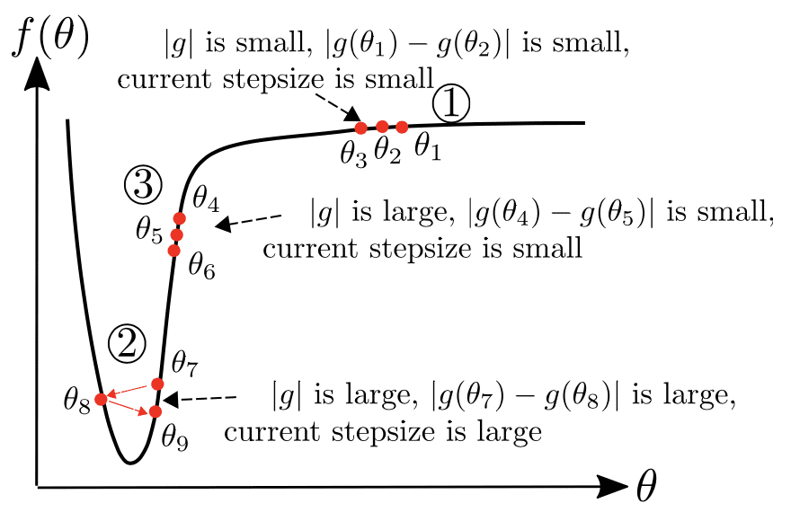
The key idea is to change the step size according to the “belief” in the current gradient direction.

But what does that mean?

In practice, we enhance Adam by computing the variance of the gradient over time instead of the momentum squared. The variance of the gradient is nothing more than the distance from the expected (believed) gradient.

In other words, v_t = \delta_2 v_{t-1} + (1-\delta_2) (\nabla_w L(x,y,w_t)^2)vt​=δ2​vt−1​+(1−δ2​)(∇w​L(x,y,wt​)2) becomes s_t = \delta_2 s_{t-1} + (1-\delta_2) (\nabla_w L(x,y,w_t) – m_t)^2 +\epsilonst​=δ2​st−1​+(1−δ2​)(∇w​L(x,y,wt​)−mt​)2+ϵ.

And that’s the only difference between AdaBelief and Adam!

That way the optimizer now considers the curvature of the loss function. If the observed gradient greatly deviates from the bilief, we distrust the current observation and take a small step.

We can think of s_tst​ as our prediction for the next gradient. If the observed gradient is close to the prediction, we trust it and take a large step. That becomes crystal clear in the below diagram where $g$ corresponds to \nabla_w L(x,y,w_t)∇w​L(x,y,wt​)

Visualizing optimizers and observations

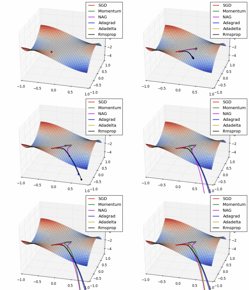
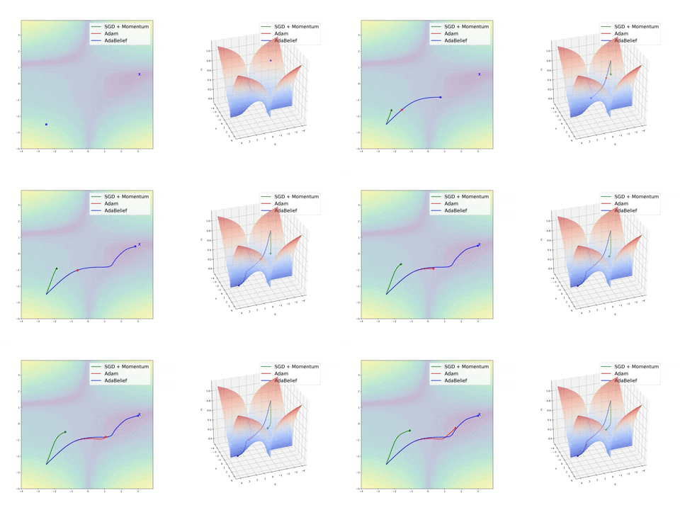
If we look at the following visualizations, the strengths and weaknesses of each algorithm become clear.

1) Algorithms with momentum have a smoother trajectory than non-momentum based but this may result in overshooting.

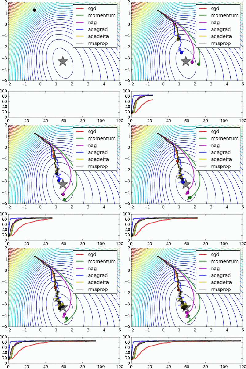
2) Methods with an adaptive learning rate have a faster convergence rate, better stability, and less jittering.

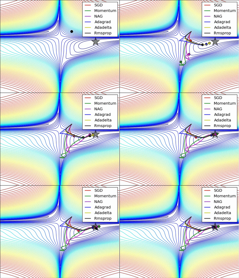
3) Algorithms that do not scale the step size (adaptive learning rate) have a harder time to escape local minimums and break the symmetry of the loss function

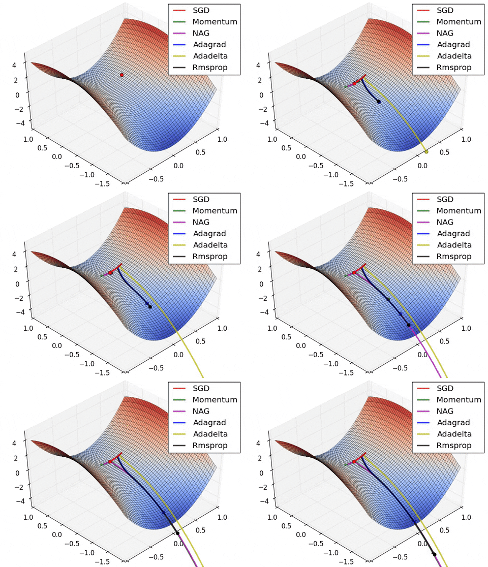
4) Saddle points cause momentum-based methods to oscillate before finding the correct downhill path

Finally, AdaBelief appears to be much faster and stable than Adam but it’s still early to jump into general conclusions

Gradient descent as an approximation of the loss function

Another way to think of optimization is as an approximation. At any given point, we try to approximate the loss function in order to move in the correct direction. Gradient descent accomplished that in a linear form. Mathematically this can be represented as a 1st-order Taylor series for the L(w) around the point w

where $d$ is the direction we’re going to move towards.

Given the above, the gradient update can be written as:

where r = -\texttt{learning\_rate} \cdot \lVert \nabla_w L(w) \rVertr=−learning_rate⋅∥∇w​L(w)∥

This intuitively tell us that Gradient Descent is simply minimizing a local approximation

For small $d$, it is obvious the approximation will be usually quite reasonable. As $d$ gets bigger, the linear approximation will start to move away from the loss function.

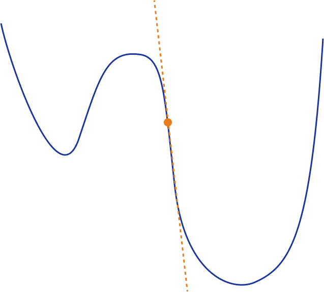
And that brings us to second-order optimization.

Second-order optimization

Naturally, a question arises in our minds. Can’t we use a higher-order approximation for better results?

By extending the above idea, we can now use a quadratic function to locally approximate our loss function. One of the most common ways to do that is to use once more a Taylor series. But this time we’ll keep both the 1st and 2nd order terms

Visually this will look like this:

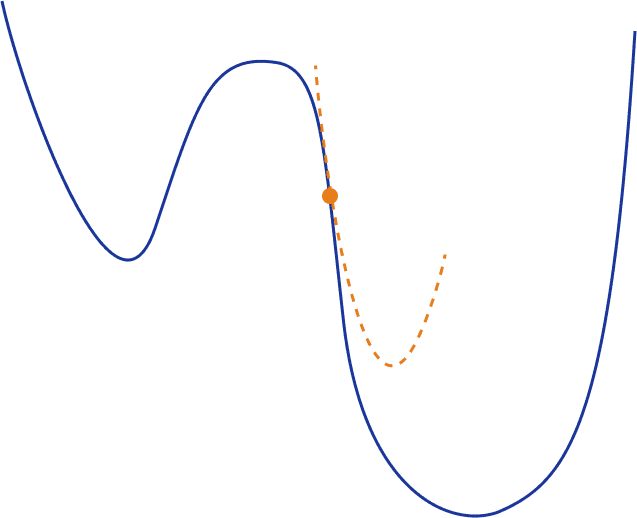
In that case, the update of the gradient will take the below form and it depends on the Hessian matrix $H(w)$:

The Hessian matrix is a square matrix of the second-order partial derivatives of a function.

Those with a mathematical background probably have already realized that this is nothing more than the well-known Newton’s method.

The rest of the algorithm remains exactly the same. Also, note that many of the aforementioned concepts such as Momentum can be applied here as well.

Shortcomings of 2nd order methods

Quadratic approximation is trustworthy only in a small local region. As we move away from the current point (large $d$), it can be very inaccurate. Thus we can’t move too fast when updating our gradients.

A common solution is to restrict the gradient updates into a local region around the point ( trust region) so we can be sure that the approximation will be fairly good. We define a region $r$ and we make sure that $|d|\le r$. Then we have:

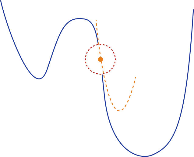
−(H(w)+λI)−1∇L(w)=argmind​(L(w)+∇w​L(w)Td+21​dT(H(w)++λI)d) where $\lambda$ depends on $r$

Another common issue is that the 2nd-order Taylor series and the Hessian matrix might not be the best quadratic approximation. In fact, this is usually true in Deep Learning applications. To overcome this, there are different alternative matrices that have been proposed. I will mention some of the most important here for completion but I will prompt you in the references section for more details:

• Empirical Fisher
• Fisher information matrix
• Gradient Covariance
• Generalized Gauss-Newton

Finally, in this category of methods, the last and biggest problem is computational complexity. Computing and storing the Hessian matrix (or any alternative matrix) requires too much memory and resources to be practical. Consider that if our weight matrix has $N$ values, the Hessian has N^2N2 values while the inverse Hessian has N^3N3. This is simply not feasible for real applications.

So what is our course of action here? Approximating the matrix with a simpler form. But how?

1. Diagonal approximation: This is the easiest approximation and is done by nullifying all non-diagonal elements of the matrix reducing the number of elements from N^2N2 to $N$. While it is computationally effective, it is likely that it will be inaccurate.
2. Block diagonal approximation: A better idea is to keep only certain diagonal blocks with the same or variable size. For example, each block might correspond to the weights of a single neuron or a single layer. The most known example is TONGA.

An example of block-diagonal is depicted below:

Results in:

3. Kronecker-product approx: A most promising approach where the aforementioned blocks correspond to the network layers. Each block is approximated by a Kronecker product of two smaller matrices. This idea is used in a powerful optimizer called K-FAC.

The Kronecker product is an operation on two matrices of arbitrary size resulting in a block matrix. It is a generalization of the outer product from vectors to matrices and gives the matrix of the tensor product with respect to a standard choice of basis.

Conclusion

In this post, we provided a complete overview of the different optimization algorithms used in Deep Learning. We started with the 3 main variations of gradient descent, we continued with the different methods proposed over the years and we concluded with second-order optimization. Optimization is still an active area of research and that’s why I will do my best to keep this article updated.

This article has been published from the source link without modifications to the text. Only the headline has been changed.

Source link