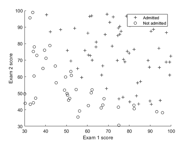
Yeah, I’m kind of a sucker for Andrew NG! Anyways, to summarize what Logistic Regression does, suppose we have the following dataset –

Figure alongside shows admission scores of students in 2 exams, and whether or not they are admitted to the school/college based on their scores. What Logistic Regression does is it tries to find a linear decision boundary that separates the classes the best.

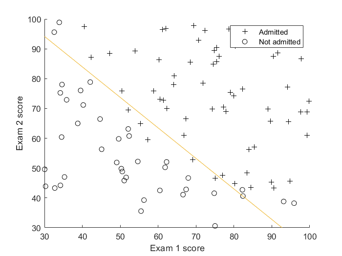
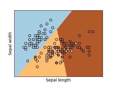
As we can see, LR does a pretty nice job separating the two classes. But what if there are more than two classes, as in our case? In that situation, we train n classifiers for each of the n classes and have each classifier try to separate one class from the rest. This technique is rightly known as the ‘one-vs-all classification’. In the end, for prediction on an instance, we pick the classifier which detects it’s class the strongest, and assign that class as the predicted class. The decision boundary here is a bit harder to visualize but here is an illustration from Sklearn –

Getting Started

Alright, enough with the requisites, now let’s get started with the code. We’ll be using Python of course, along with the following modules: Numpy, Matplotlib, Seaborn and Sklearn. In case if like work locally on your computer like me, make sure you have these modules installed. To install them, simply fire up your Command Line/Terminal and enter the command “pip install <module-name>”. To check what modules are installed, enter “python” then “help(‘modules’)” to generate list of all installed modules.

Data Analysis And Visualization

First, we need to get an idea of the distribution of data in the dataset. Let’s import the matplotlib and seaborn modules for this purpose and load the iris dataset contained in the seaborn module.

import matplotlib.pyplot as plt
import seaborn as sns
iris = sns.load_dataset(‘iris’)

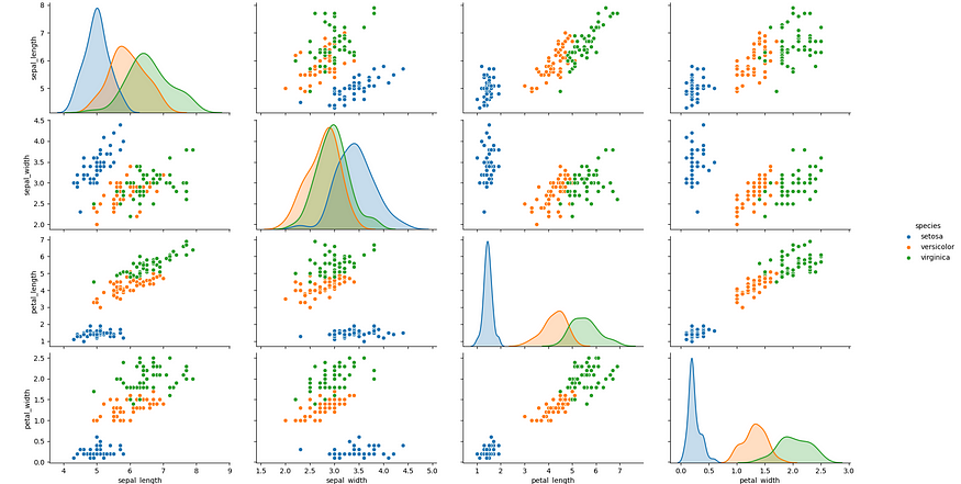
This will load the dataset into the dataframe ‘iris’, which will make visualization much easier. Since the dataset has 4 features we can’t visualize it directly but we can gain some intuition through seaborn’s powerful pairplot. What pairplot does is it makes a scatter plot between each of the pairs of variables in the dataset, as well as the distribution of values of each variable (along the diagonal graphs). This can be used to analyze which features are a better separator of the data, which features are closely related, as well as data distribution.

sns.pairplot(iris, hue='species') #hue parameter colors distinct species
plt.show()

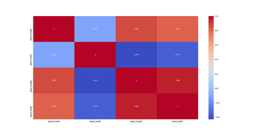
Another powerful tool in Seaborn is the heatmap of correlations. Correlation is a statistical measure of how much two variables are dependent on each other. If an increase in one variable causes a rough increase in another variable and vice versa, then they are said to be positively correlated. If an increase in a variable causes a decrease in another and vice versa, they are negatively correlated and if there is no such dependence between them, they have zero correlation. This is how we plot correlations using Seaborn –

sns.heatmap(iris.corr(), annot=True, cmap='coolwarm')
plt.show()

iris.corr() generates a 4*4 matrix with each entry (i,j) representing correlations between the iᵗʰ and jᵗʰ variables. Obviously the matrix is symmetric, since the dependence between i and j is same as that between j and i (wish this were true for humans too). And the diagonal elements are 1, since a variable is obviously completely dependent on itself. The annot parameter decides whether to display the correlation values on top of the heatmap and colormap is set to coolwarm, which means blue for low values and red for high values.

Data Preparation And Preprocessing

Now that we have an intuition about the data, let’s load the data into numpy arrays and preprocess it. Preprocessing is a crucial step and can enhance the performance of your algorithms by a huge margin. We import the required modules, load the dataset from sklearn’s iris datasets class in the form of a dictionary, get the features and targets into numpy arrays X and Y, respectively and the names of the classes into names. Since the targets specified in the datasets are 0,1 and 2 representing the 3 classes of species, we would like a mapping from those integers to the name of the class they represent. To do this, we create a dictionary mapping from the integers 0,1,2 to the flower names.

import numpy as np
from sklearn.datasets import load_iris
dataset = load_iris()
X, Y, names = dataset['data'], dataset['target'], dataset['target_names']
target = dict(zip(np.array([0, 1, 2]), names))

Let’s move forward to the preprocessing step. We divide the data into train and test sets using train_test_split from sklearn using test set size of 25%, then use the StandardScaler class from sklearn. What StandardScaler does is it computes the mean and standard deviation of each of the features in our dataset, then subtracts off the mean and divides by the standard deviation each example in our dataset. This brings all of the features to having zero mean and unit standard deviation/variance. Bringing all of the features in the same range is also known as feature normalization, and it helps optimization algorithms like gradient descent to work properly and converge faster.

from sklearn.preprocessing import StandardScaler
from sklearn.model_selection import train_test_split
X_train, X_test, Y_train, Y_test = train_test_split(X, Y, test_size=0.25)
scaler = StandardScaler()  #create object of StandardScaler class
scaler.fit(X_train)        #fit it to the training set
X_train_pr = scaler.transform(X_train) #apply normalization to the training set

Building The Model And Evaluating It

It’s time for the real deal. It is now that you feel really indebted to sklearn for making your life simple. We create an object of the LogisticRegression class named model, and fit our training dataset to it, all using 3 lines of code –

from sklearn.linear_model import LogisticRegression
model = LogisticRegression()
model.fit(X_train_pr, Y_train)

Now, to make predictions we first normalize the test set using the Standard Scaler. Note that the transformation is the same as applied to the training set (to which we had fit the scaler to). This is important as we have to normalize our test set as per the mean and standard deviation of our training set, and not the test set. We then use the predict function to generate the 1D array of predictions both on the training and test set. There are many metrics available in the metrics class of sklearn but we’ll use the 3 most relevant — accuracy, classification report and confusion matrix.

from sklearn.metrics import accuracy_score, classification_report, confusion_matrix
X_test_pr = scaler.transform(X_test)
Y_train_pred, Y_test_pred = model.predict(X_train_pr), model.predict(X_test_pr) 
print(accuracy_score(Y_train, Y_train_pred))
print(accuracy_score(Y_test, Y_test_pred))
print(classification_report(Y_test, Y_test_pred))
print(confusion_matrix(Y_test, Y_test_pred))

The dataset is very small, and hence, you might very different results each time you train your model. This is the output I get –

In case if you don’t understand any of the metrics you see, feel free to search them they are pretty much basic and easy to understand. Training set accuracy is approx 95.5% and test set accuracy approx 94.7%. A weighted average of F1-score of all different classes in the test set is 0.95 and 2 examples from the test set are classified incorrectly. An accuracy of 94.7% on the training set at first go is really good, but we can do better.

Improving The Model

Let’s introduce polynomial logistic regression. It turns out that we can build a better model by introducing polynomial features into the model, like x₁², x₁x₂, x₂² to produce a non-linear decision boundary to better separate the classes. This kind of model is more practical. For example, let us look at this dataset below –

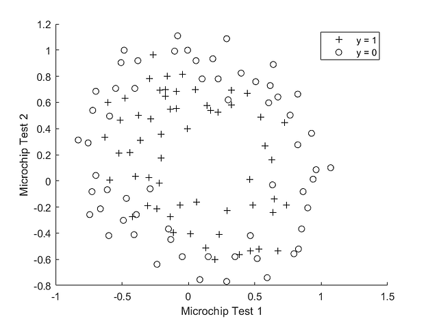
This dataset looks a little more practical, doesn’t it? It shows scores achieved by tests on different microchips and the classes they belong to. There is clearly no linear decision boundary that can satisfactorily separate the data. Using polynomial logistic regression, we can get a decision boundary as shown below, which does a far better job.

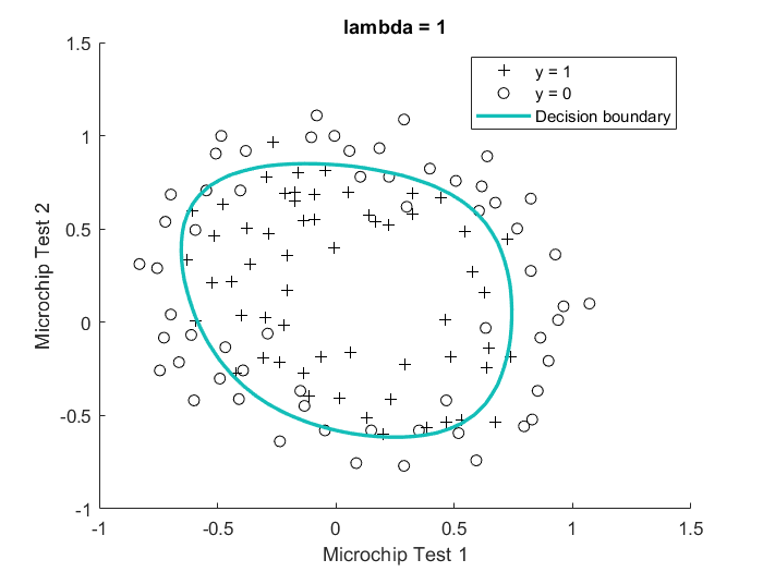
The lambda=1 in the figure refers to the regularization parameter. Regularization become pretty important when dealing with non-linear models since you don’t want to overfit to your training set and have your model not perform well on new examples it hasn’t seen.

To add polynomial features into your dataset, we use the PolynomialFeatures class from sklearn. This will go into your preprocessing as an added step, similar to the feature normalization step. We add 5th power degree terms, you can try changing it and see the effect it has on your accuracy. It turns out the model starts overfitting for higher degree terms and we don’t want that.

from sklearn.preprocessing import PolynomialFeatures
X_train, X_test, Y_train, Y_test = train_test_split(X, Y, test_size=0.25)
poly = PolynomialFeatures(degree = 5)
poly.fit(X_train)
X_train_pr = poly.transform(X_train)
scaler = StandardScaler()
scaler.fit(X_train_pr)
X_train_pr = scaler.transform(X_train_pr)

Then continue the same steps as discussed above to fit the model. To make predictions, don’t forget to transform the test set using poly first.

X_test_pr = poly.transform(X_test)
X_test_pr = scaler.transform(X_test_pr)
Y_train_pred, Y_test_pred = model.predict(X_train_pr), model.predict(X_test_pr)

Then evaluate the model, using the metrics discussed above. Again, the results will differ with each time the model is trained. Here is my output –

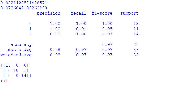
Pretty good results! A training set accuracy of approx 98.2% and a test set accuracy of approx 97.4% are great using a simple algorithm like logistic regression. Weighted F1-score on test set has improved to 0.97 and the model incorrectly classifies only 1 example from the test set.

Generating Predictions

It’s time to use the model to generate predictions. We’ll give it an array of 4 numbers — representing the 4 features of a flower, and it will tell us which species it thinks that it belongs to. We randomly pick 20 examples from the dataset, preprocess them and get the predicted classes.

indices = np.random.randint(150, size=20)
X_pred, Y_true = X[indices], Y[indices]
X_pred_pr = poly.transform(X_pred)
X_pred_pr = scaler.transform(X_pred_pr)
Y_pred = model.predict(X_pred_pr)

Note that Y_true represents the true class of the example and Y_pred is the predicted class. They are both integers as the model works with numeric data. We will now create 2 lists, storing the true names and predicted names of the species of each example, using the dictionary mapping we already created named target.

target_true, target_pred = [], []
for i in range(len(Y_true)):
    target_true.append(target[Y_true[i]])
    target_pred.append(target[Y_pred[i]])
print(X_pred)
print(target_true)
print(target_pred)

This is the output I get –

Due to the high accuracy of our model, all the 20 predictions generated are correct! Here is the complete code of the final model we created –

import numpy as np
import matplotlib.pyplot as plt
import seaborn as sns
from sklearn.datasets import load_iris
from sklearn.preprocessing import PolynomialFeatures, StandardScaler
from sklearn.model_selection import train_test_split
from sklearn.metrics import accuracy_score, classification_report, confusion_matrix
from sklearn.linear_model import LogisticRegression

dataset = load_iris()
X, Y, names = dataset['data'], dataset['target'], dataset['target_names']
target = dict(zip(np.array([0, 1, 2]), names))
iris = sns.load_dataset('iris')
sns.pairplot(iris, hue='species')
plt.show()
sns.heatmap(iris.corr(), annot=True, cmap='coolwarm')
plt.show()
X_train, X_test, Y_train, Y_test = train_test_split(X, Y, test_size=0.25)
poly = PolynomialFeatures(degree = 5)
poly.fit(X_train)
X_train_pr = poly.transform(X_train)
scaler = StandardScaler()
scaler.fit(X_train_pr)
X_train_pr = scaler.transform(X_train_pr)
model = LogisticRegression()
model.fit(X_train_pr, Y_train)

X_test_pr = poly.transform(X_test)
X_test_pr = scaler.transform(X_test_pr)
Y_train_pred, Y_test_pred = model.predict(X_train_pr), model.predict(X_test_pr) 
print(accuracy_score(Y_train, Y_train_pred))
print(accuracy_score(Y_test, Y_test_pred))
print(classification_report(Y_test, Y_test_pred))
print(confusion_matrix(Y_test, Y_test_pred))

indices = np.random.randint(150, size=20)
X_pred, Y_true = X[indices], Y[indices]
X_pred_pr = poly.transform(X_pred)
X_pred_pr = scaler.transform(X_pred_pr)
Y_pred = model.predict(X_pred_pr)
target_true, target_pred = [], []
for i in range(len(Y_true)):
    target_true.append(target[Y_true[i]])
    target_pred.append(target[Y_pred[i]])
print(X_pred)
print(target_true)
print(target_pred)