In the following weeks, I will post a series of tutorials giving comprehensive introductions into unsupervised and self-supervised learning using neural networks for the purpose of image generation, image augmentation, and image blending. The topics include:
- Variational Autoencoders (VAEs) (this tutorial)
- Neural Style Transfer Learning
- Generative Adversarial Networks (GANs)
For this tutorial, we focus on a specific type of autoencoder called a variational autoencoder. There are several articles online explaining how to use autoencoders, but none are particularly comprehensive in nature. In this article, I plan to provide the motivation for why we might want to use VAEs, as well as the kinds of problems they solve, to give mathematical background into how these neural architectures work, and some real-world implementations using Keras.
This article borrows content from lectures taken at Harvard on AC209b, and major credit should go to lecturer Pavlos Protopapas of the Harvard IACS department.
VAEs are arguably the most useful type of autoencoder, but it is necessary to understand traditional autoencoders used for typically for data compression or denoising before we try to tackle VAEs.
First, though, I will try to get you excited about the things VAEs can do by looking at a few examples.
The power of VAEs
Let’s say you are developing a video game, and you have an open-world game that has very complex scenery. You hire a team of graphic designers to make a bunch of plants and trees to decorate your world with, but once putting them in the game you decide it looks unnatural because all of the plants of the same species look exactly the same, what can you do about this?
At first, you might suggest using some parameterizations to try and distort the images randomly, but how many features would be enough? How large should this variation be? And an important question, how computationally intensive would it be to implement?
This is an ideal situation to use a variational autoencoder. We can train a neural network to learn latent features about the plant, and then every time one pops up in our world, we can take a random sample from our “learned” features and generate a unique plant. This is, in fact, how many open world games have started to generate aspects of the scenery within their worlds.
Let’s go for a more graphical example. Imagine we are an architect and want to generate floor plans for a building of arbitrary shape. We can an autoencoder network to learn a data generating distribution given an arbitrary build shape, and it will take a sample from our data generating distribution and produce a floor plan. This idea is shown in the animation below.
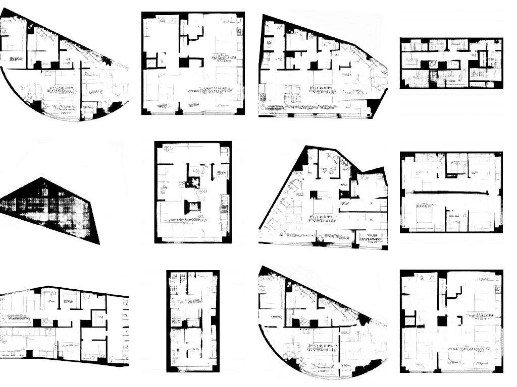
The potential of these for designers is arguably the most prominent. Imagine instead we work for a fashion company and are tasked with creating new styles of clothing, we could, in fact, just train an autoencoder on “fashionable” items and allow the network to learn a data generating distribution for fashionable clothing. Subsequently, we can take samples from this low-dimensional latent distribution and use this to create new ideas.
This final example is the one that we will work with during the final section of this tutorial, where will study the fashion MNIST dataset.
Autoencoders
Traditional Autoencoders
Autoencoders are surprisingly simple neural architectures. They are basically a form of compression, similar to the way an audio file is compressed using MP3, or an image file is compressed using JPEG.
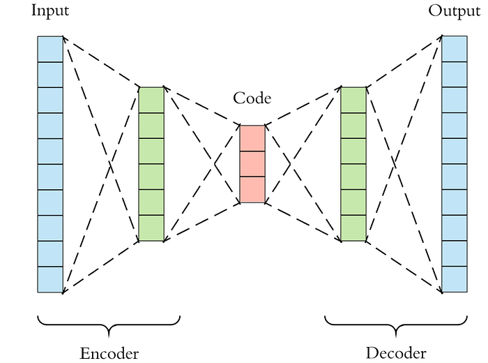
Autoencoders are closely related to principal component analysis (PCA). In fact, if the activation function used within the autoencoder is linear within each layer, the latent variables present at the bottleneck (the smallest layer in the network, aka. code) directly correspond to the principal components from PCA. Generally, the activation function used in autoencoders is non-linear, typical activation functions are ReLU (Rectified Linear Unit) and sigmoid.
The math behind the networks is fairly easy to understand, so I will go through it briefly. Essentially, we split the network into two segments, the encoder, and the decoder.
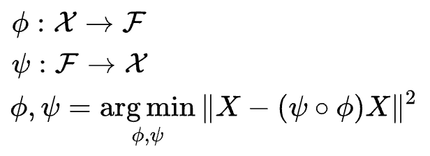
The encoder function, denoted by ϕ, maps the original data X, to a latent space F, which is present at the bottleneck. The decoder function, denoted by ψ, maps the latent space F at the bottleneck to the output. The output, in this case, is the same as the input function. Thus, we are basically trying to recreate the original image after some generalized non-linear compression.
The encoding network can be represented by the standard neural network function passed through an activation function, where z is the latent dimension.

Similarly, the decoding network can be represented in the same fashion, but with different weight, bias, and potentially activation functions being used.

The loss function can then be written in terms of these network functions, and it is this loss function that we will use to train the neural network through the standard backpropagation procedure.

Since the input and output are the same images, this is not really supervised or unsupervised learning, so we typically call this self-supervised learning. The aim of the autoencoder is to select our encoder and decoder functions in such a way that we require the minimal information to encode the image such that it be can regenerated on the other side.
If we use too few nodes in the bottleneck layer, our capacity to recreate the image will be limited and we will regenerate images that are blurry or unrecognizable from the original. If we use too many nodes, then there is little point in using compression at all.
The case for compression is pretty simple, whenever you download something on Netflix, for example, the data that is sent to you is compressed. Once it arrives at your computer, it is passed through a decompression algorithm and then displayed on your computer. This is analogous to how zip files work, except it is done behind the scenes via a streaming algorithm.
Denoising Autoencoders
There are several other types of autoencoders. One of the most commonly used is a denoising autoencoder, which will analyze with Keras later in this tutorial. These autoencoders add some white noise to the data prior to training but compare the error to the original image when training. This forces the network to not become overfit to arbitrary noise present in images. We will use this later to remove creases and darkened areas from scanned images of documents.
Sparse Autoencoders
A sparse autoencoder, counterintuitively, has a larger latent dimension than the input or output dimensions. However, each time the network is run, only a small fraction of the neurons fires, meaning that the network is inherently ‘sparse’. This is similar to a denoising autoencoder in the sense that it is also a form of regularization to reduce the propensity for the network to overfit.
Contractive Autoencoder
Contractive encoders are much the same as the last two procedures, but in this case, we do not alter the architecture and simply add a regularizer to the loss function. This can be thought of as a neural form of ridge regression.
So now that we understand how autoencoders are, we need to understand what they are not good at. Some of the biggest challenges are:
- Gaps in the latent space
- Separability in the latent space
- Discrete latent space
These problems can all be illustrated in this diagram.
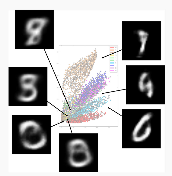
This diagram shows us the location of different labeled numbers within the latent space. We can see that the latent space contains gaps, and we do not know what characters in these spaces may look like. This is equivalent to having a lack of data in a supervised learning problem, as our network has not been trained for these circumstances of the latent space. Another issue is the separability of the spaces, several of the numbers are well separated in the above figure, but there are also regions where the labeled is randomly interspersed, making it difficult to separate the unique features of characters (in this case the numbers 0–9). Another issue here is the inability to study a continuous latent space, for example, we do not have a statistical model that has been trained for arbitrary input (and would not even if we closed all gaps in the latent space).
These issues with traditional autoencoders mean that we still have a way to go before we can learn the data generating distribution and produce new data and images.
Now that we understand how traditional autoencoders work, we will move on to variational autoencoders. These are slightly more complex as they implement a form of variational inference taken from Bayesian statistics. We will discuss this in more depth in the next section
Variational Autoencoders
VAEs inherit the architecture of traditional autoencoders and use this to learn a data generating distribution, which allows us to take random samples from the latent space. These random samples can then be decoded using the decoder network to generate unique images that have similar characteristics to those that the network was trained on.

For those of you familiar with Bayesian statistics, the encoder is learning an approximation to the posterior distribution. This distribution is typically intractable to do analytically since it does not have a closed form solution. This means that we can either perform computationally expensive sampling procedures such as Markov Chain Monte Carlo (MCMC) methods, or we can use variational methods. The variational autoencoder, as one might suspect, uses variational inference to generate its approximation to this posterior distribution.
We will discuss this procedure in a reasonable amount of detail, but for the in-depth analysis, I highly recommend checking out the blog post by Jaan Altosaar. Variational inference is a topic for a graduate machine learning or statistics class, but you do not need a degree in statistics to understand the basic ideas. Here is a link to Jaan’s article for those interested:
For those of you not interested in the underlying mathematics, feel free to skip to the VAE coding tutorial.
The first thing we need to understand is the posterior distribution and why we cannot calculate it. Take a look at the equation below, this is Bayes’ theorem. The premise here is that we want to know how to learn how to generate data, x, from our latent variables, z. This implies that we want to learn p(z|x). Unfortunately, we do not know this distribution, but we do not need to since we can reformulate this probability with Bayes’ theorem. This does not solve all of our problems, however, as the denominator, known as the evidence, is often intractable. All is not lost though, as a cheeky solution exists that allows us to approximate this posterior distribution. It turns out we can cast this inference problem into an optimization problem.

In order to approximate the posterior distribution, we need a way of assessing how good a proposal distribution is compared to the true posterior. To do this, we use a Bayesian statistician’s best friend, the Kullback-Leibler divergence. The KL divergence is a measure of how similar two probability distributions are; if they are the same, the divergence is zero, and if it is a positive number, the two distributions are different. The KL divergence is strictly positive, although it is technically not a distance because the function is not symmetric. We use the KL divergence in the following manner.

This equation may look intimidating, but the idea here is quite simple. We propose a family of possible distributions that could possibly be how our data was generated, Q, and we want to find the optimal distribution, q*, which minimizes our distance between the proposed distribution and the actual distribution, which we are trying to approximate due to its intractability. We still have one problem with this formula, namely, that we do not actually know p(z|x), so we cannot calculate the KL divergence. How do we resolve this?
This is where things get a little bit esoteric. We can do some mathematical manipulation and rewrite the KL divergence in terms of something called the ELBO (Evidence Lower Bound) and another term involving p(x).

What is interesting here is that the ELBO is the only variable in this equation that depends on what distribution we select. The other term is not influenced by our choice of distribution since it does not depend on q. Thus, we can minimize the KL divergence by maximizing (since it is negative) the ELBO in the above equation. The key point of this is that we can actually calculate the ELBO, meaning we can now perform an optimization procedure.
So all we need to do now is come up with a good choice for Q and then differentiate the ELBO, set it to zero and voila, we have our optimal distribution. There are a few more snags before this is possible, first, we have to decide what is a good family of distributions to select.
Typically, mean field variational inference is done for simplicity when defining q. This essentially says that each variational parameter is independent of each other. We, therefore, have a single q for each data point, which we can multiply together to give a joint probability, giving us the ‘mean field’ q.

In reality, we could select as many fields, or clusters, as we would like. In the case of MNIST, for example, we might select 10 clusters since we know that there are 10 possible numbers that could be present.
The second thing we need to do is something often known as the reparameterization trick, whereby we take the random variables outside of the derivative since taking the derivative of a random variable gives us much larger errors due to their inherent randomness.
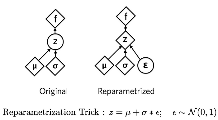
The reparameterization trick is a little esoteric, but it basically says that I can write a normal distribution as a mean plus some standard deviation, multiplied by some error. This means that when differentiating, we are not taking the derivative of the random function itself, merely its parameters.
If that did not make much sense, here is a good article that explains the trick and why it performs better than taking derivatives of the random variables themselves:
This procedure does not have a general closed-form solution, so we are still somewhat constrained in our ability to approximate the posterior distribution. However, the exponential family of distributions does, in fact, have a closed form solution. This means that we can use standard distributions, such as the normal distribution, binomial, Poisson, beta, etc. So, whilst we may not find the true posterior distribution, we can find an approximation which does the best job given the exponential family of distributions.
The art of variational inference is selecting our family of distributions, Q, to be large enough to get a good approximation of the posterior, but not too large that it takes an excessively long time to compute.
Now that we have a decent idea of how our network has been trained to learn the latent distribution of our data, we can look at how we generate data using this distribution.
The Data Generating Procedure
Looking at the below image, we can consider that our approximation to the data generating procedure decides that we want to generate the number ‘2’, so it generates the value 2 from the latent variable centroid. However, we may not want to generate the same looking ‘2’ every time, as in our video game example with plants, so we add some random noise to this item in the latent space, which is based on a random number and the ‘learned’ spread of the distribution for the value ‘2’. We pass this through our decoder network and we get a 2 which looks different to the original.
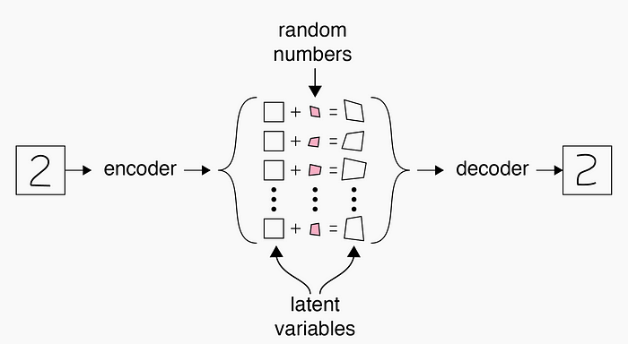
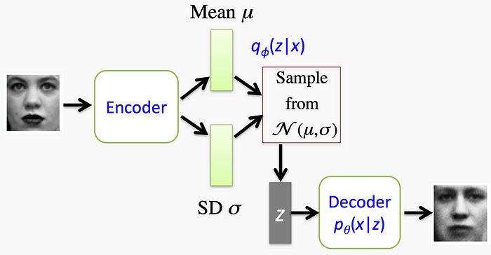
This was an oversimplified version which abstracted the architecture of the actual autoencoder network. Below is a representation of the architecture of a real variational autoencoder using convolutional layers in the encoder and decoder networks. We see that we are learning the centers and spreads of the data generating distributions within the latent space separately, and then ‘sampling’ from these distributions to generate essentially ‘fake’ data.

The inherent nature of the learning procedure means that parameters that look similar (stimulate the same network neurons to fire) are clustered together in the latent space, and are not spaced arbitrarily. This is illustrated in the figure below. We see that our values of 2’s begin to cluster together, whilst the value 3 gradually becomes pushed away. This is useful as it means the network does not arbitrarily place characters in the latent space, making the transitions between values less spurious.
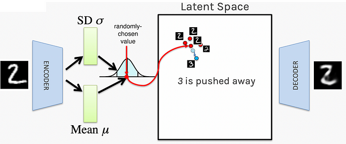
An overview of the entire network architecture is shown below. Hopefully, at this point, the procedure makes sense. We train the autoencoder using a set of images to learn our mean and standard deviations within the latent space, which forms our data generating distribution. Next, when we want to generate a similar image, we sample from one of the centroids within the latent space, distort it slightly using our standard deviation and some random error, and then pass this through the decoder network. It is clear from this example that the final output looks similar, but not the same, as the input image.
VAE Coding Tutorial
In this section, we will look at a simple denoising autoencoder for removing creases and marks on scanned images of documents, as well as removing noise within the fashion MNIST dataset. We will then use VAEs to generate new items of clothing after training the network on the MNIST dataset.
Denoising Autoencoders
Fashion MNIST
For the first exercise, we will add some random noise (salt and pepper noise) to the fashion MNIST dataset, and we will attempt to remove this noise using a denoising autoencoder. First, we perform our preprocessing: download the data, scale it, and then add our noise.
## Download the data
(x_train, y_train), (x_test, y_test) = datasets.fashion_mnist.load_data()

## normalize and reshape
x_train = x_train/255.
x_test = x_test/255.

x_train = x_train.reshape(-1, 28, 28, 1)
x_test = x_test.reshape(-1, 28, 28, 1)

# Lets add sample noise - Salt and Pepper
noise = augmenters.SaltAndPepper(0.1)
seq_object = augmenters.Sequential([noise])

train_x_n = seq_object.augment_images(x_train * 255) / 255
val_x_n = seq_object.augment_images(x_test * 255) / 255
After this, we create the architecture for our autoencoder network. This involves multiple layers of convolutional neural networks, max-pooling layers on the encoder network, and upscaling layers on the decoder network.
# input layer
input_layer = Input(shape=(28, 28, 1))

# encoding architecture
encoded_layer1 = Conv2D(64, (3, 3), activation='relu', padding='same')(input_layer)
encoded_layer1 = MaxPool2D( (2, 2), padding='same')(encoded_layer1)
encoded_layer2 = Conv2D(32, (3, 3), activation='relu', padding='same')(encoded_layer1)
encoded_layer2 = MaxPool2D( (2, 2), padding='same')(encoded_layer2)
encoded_layer3 = Conv2D(16, (3, 3), activation='relu', padding='same')(encoded_layer2)
latent_view    = MaxPool2D( (2, 2), padding='same')(encoded_layer3)

# decoding architecture
decoded_layer1 = Conv2D(16, (3, 3), activation='relu', padding='same')(latent_view)
decoded_layer1 = UpSampling2D((2, 2))(decoded_layer1)
decoded_layer2 = Conv2D(32, (3, 3), activation='relu', padding='same')(decoded_layer1)
decoded_layer2 = UpSampling2D((2, 2))(decoded_layer2)
decoded_layer3 = Conv2D(64, (3, 3), activation='relu')(decoded_layer2)
decoded_layer3 = UpSampling2D((2, 2))(decoded_layer3)
output_layer   = Conv2D(1, (3, 3), padding='same', activation='sigmoid')(decoded_layer3)

# compile the model
model = Model(input_layer, output_layer)
model.compile(optimizer='adam', loss='mse')

# run the model
early_stopping = EarlyStopping(monitor='val_loss', min_delta=0, patience=10, verbose=5, mode='auto')
history = model.fit(train_x_n, x_train, epochs=20, batch_size=2048, validation_data=(val_x_n, x_test), callbacks=[early_stopping])
The model takes a while to run unless you have a GPU, it can take around 3–4 minutes per epoch. Our input images, input images with noise, and our output images are shown below.


As you can see, we are able to remove the noise adequately from our noisy images, but we have lost a fair amount of resolution of the finer features of the clothing. This is one of the prices we pay for a robust network. The network can be tuned in order to make this final output more representative of the input images.
Text Cleaning
Our second example with denoising autoencoders involves cleaning scanned images of creases and dark areas. Here are our input and output images that we would like to obtain.
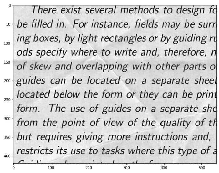
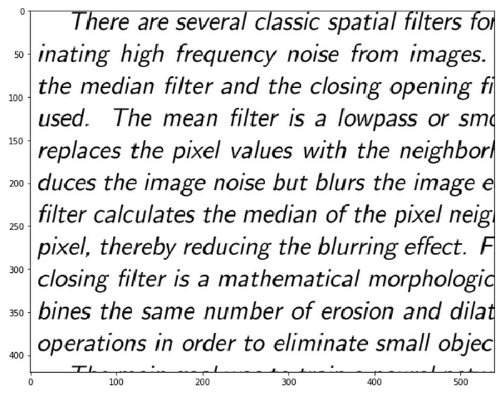
The data preprocessing for this is a bit more involved, and so I will not introduce that here, but it is available on my GitHub repository, along with the data itself. The network architecture is as follows.
input_layer = Input(shape=(258, 540, 1))

# encoder
encoder = Conv2D(64, (3, 3), activation='relu', padding='same')(input_layer)
encoder = MaxPooling2D((2, 2), padding='same')(encoder)

# decoder
decoder = Conv2D(64, (3, 3), activation='relu', padding='same')(encoder)
decoder = UpSampling2D((2, 2))(decoder)
output_layer = Conv2D(1, (3, 3), activation='sigmoid', padding='same')(decoder)

ae = Model(input_layer, output_layer)

ae.compile(loss='mse', optimizer=Adam(lr=0.001))

batch_size = 16
epochs = 200

early_stopping = EarlyStopping(monitor='val_loss',min_delta=0,patience=5,verbose=1, mode='auto')
history = ae.fit(x_train, y_train, batch_size=batch_size, epochs=epochs, validation_data=(x_val, y_val), callbacks=[early_stopping])
Variational Autoencoders
For our finale, we will try to generate new images of clothing items that are present in the fashion MNIST dataset.
The neural architecture for this is a little bit more complicated, and contains a sampling layer called a ‘Lambda’ layer.
batch_size = 16
latent_dim = 2  # Number of latent dimension parameters

# ENCODER ARCHITECTURE: Input -> Conv2D*4 -> Flatten -> Dense
input_img = Input(shape=(28, 28, 1))

x = Conv2D(32, 3,
                  padding='same',
                  activation='relu')(input_img)
x = Conv2D(64, 3,
                  padding='same',
                  activation='relu',
                  strides=(2, 2))(x)
x = Conv2D(64, 3,
                  padding='same',
                  activation='relu')(x)
x = Conv2D(64, 3,
                  padding='same',
                  activation='relu')(x)

# need to know the shape of the network here for the decoder
shape_before_flattening = K.int_shape(x)

x = Flatten()(x)
x = Dense(32, activation='relu')(x)

# Two outputs, latent mean and (log)variance
z_mu = Dense(latent_dim)(x)
z_log_sigma = Dense(latent_dim)(x)

## SAMPLING FUNCTION

def sampling(args):
    z_mu, z_log_sigma = args
    epsilon = K.random_normal(shape=(K.shape(z_mu)[0], latent_dim),
                              mean=0., stddev=1.)
    return z_mu + K.exp(z_log_sigma) * epsilon

# sample vector from the latent distribution
z = Lambda(sampling)([z_mu, z_log_sigma])

## DECODER ARCHITECTURE

# decoder takes the latent distribution sample as input
decoder_input = Input(K.int_shape(z)[1:])

# Expand to 784 total pixels
x = Dense(np.prod(shape_before_flattening[1:]),
                 activation='relu')(decoder_input)

# reshape
x = Reshape(shape_before_flattening[1:])(x)

# use Conv2DTranspose to reverse the conv layers from the encoder
x = Conv2DTranspose(32, 3,
                           padding='same',
                           activation='relu',
                           strides=(2, 2))(x)
x = Conv2D(1, 3,
                  padding='same',
                  activation='sigmoid')(x)

# decoder model statement
decoder = Model(decoder_input, x)

# apply the decoder to the sample from the latent distribution
z_decoded = decoder(z)
This is the architecture, but we still need to insert the loss function and incorporate the KL divergence.
# construct a custom layer to calculate the loss
class CustomVariationalLayer(Layer):

    def vae_loss(self, x, z_decoded):
        x = K.flatten(x)
        z_decoded = K.flatten(z_decoded)
        # Reconstruction loss
        xent_loss = binary_crossentropy(x, z_decoded)
        # KL divergence
        kl_loss = -5e-4 * K.mean(1 + z_log_sigma - K.square(z_mu) - K.exp(z_log_sigma), axis=-1)
        return K.mean(xent_loss + kl_loss)

    # adds the custom loss to the class
    def call(self, inputs):
        x = inputs[0]
        z_decoded = inputs[1]
        loss = self.vae_loss(x, z_decoded)
        self.add_loss(loss, inputs=inputs)
        return x

# apply the custom loss to the input images and the decoded latent distribution sample
y = CustomVariationalLayer()([input_img, z_decoded])

# VAE model statement
vae = Model(input_img, y)
vae.compile(optimizer='rmsprop', loss=None)

vae.fit(x=train_x, y=None,
        shuffle=True,
        epochs=20,
        batch_size=batch_size,
        validation_data=(val_x, None))
We can now view our reconstructed samples to see what our network was able to learn.
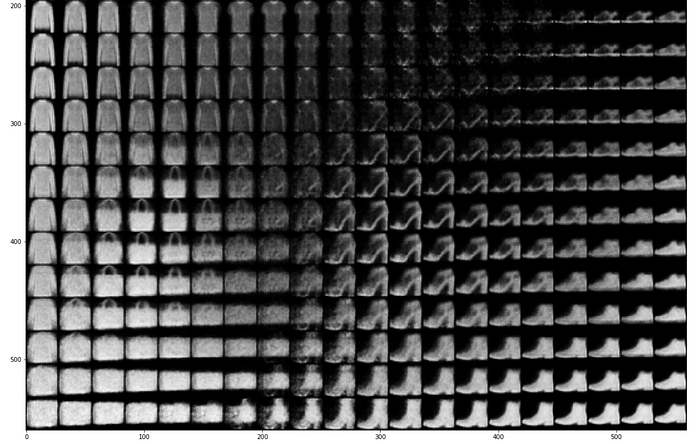
We can clearly see transitions between shoes, handbags, as well as clothing items. Not all of the latent space is plotted here to help with image clarity. We can also view the latent space and color code each of the 10 clothing items present in the fashion MNIST dataset.
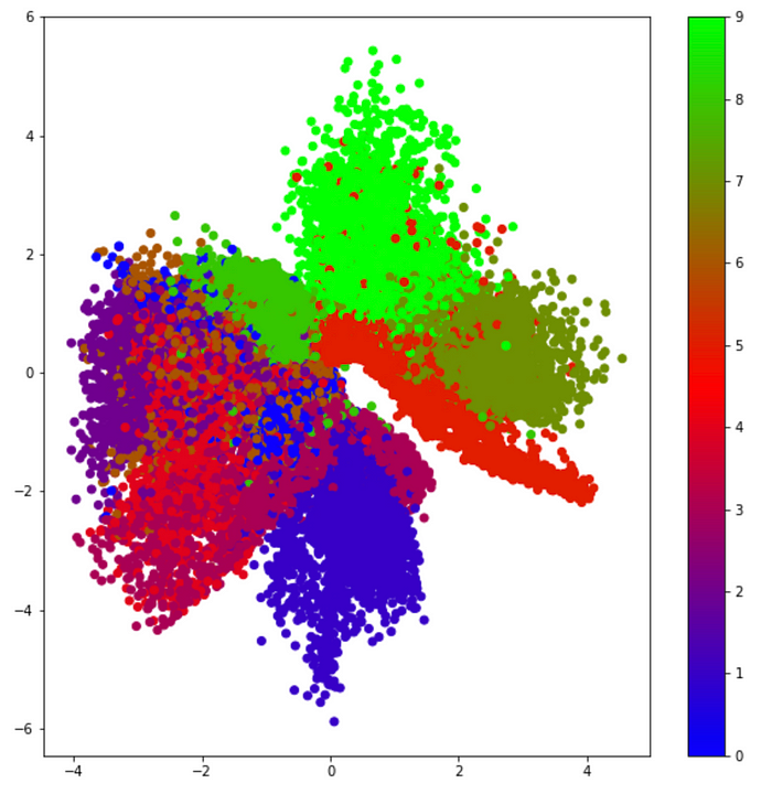
We see that the items are separated into distinct clusters.
Final Comments
This tutorial was a crash course in autoencoders, variational autoencoders, and variational inference. I hope that the reader found this interesting, and now has a better understanding of what autoencoders are and how they can be used in real-world applications.
This article has been published from the source link without modifications to the text. Only the headline has been changed.
Source link


