An overview of Dimensionality Reduction methods — Correlation, PCA, t-SNE, Autoencoders and their implementation in python

Dimensionality Reduction is the process of reducing the number of features or variables in the dataset. It is the transformation of data from a high-dimensional space into a low-dimensional space so that the low-dimensional representation retains some meaningful properties of the original data.

Why Dimensionality Reduction is important?

In real-world datasets, there are often too many variables in the data. The higher the number of features, the harder it gets to visualize the data and work on it. Sometimes, most of these features are correlated, and hence redundant. This is where dimensionality reduction algorithms come into play.

There are various methods to reduce the dimensionality of the data, in this article you can understand some of them:

1. Feature Selection Methods: Using Correlation Coefficient Methods
2. Matrix Factorization: PCA
3. Manifold Learning: t-SNE
4. Auto Encoders

Feature Selection Methods:

Some of the datasets have a large number of features, and only some of these features are correlated with the target class label. Feature selection techniques use scoring or statistical methods to select which features to keep and which features to delete.

Techniques or algorithms used to reduce dimensions by selecting top features are:

• Pearson Correlation Coefficient (numerical input, numerical output)
• Spearman Correlation Coefficient (numerical input, numerical output)
• Chi-Squared Test (categorical input, categorical output)
• Kendall Tau Test (numerical input, categorical output)

Depending on whether features of training data are numerical or categorical and whether the target class label is numerical or categorical, different features selection from the above list can be chosen.

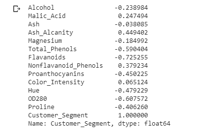
For a sample wine dataset taken from UCI ML Repository. The target class label is categorical and the rest of the training data is having numerical features. So we can find the top features which are highly correlated to the target class label (“Customer_Segment”) using the Kendall Tau Test.

import pandas as pd

data = pd.read_csv("Wine.csv")
print(data.corr(method="kendall")["Customer_Segment"])

From the above Kendall coefficient of each feature in the dataset with target class label “Customer_Segment”, it is confirmed that features “Flavanoids”, “OD280”, and “Total_Phenols” are top 3 features having maximum modular value. You can pick top x features by taking the modulo of coefficient values.

Matrix Factorization:

Matrix Factorization methods can be used for dimension reduction. Principal Component Analysis (PCA) is a matrix factorization technique to reduce higher dimension data to lower dimensions. PCA preserves the direction with maximal variance.

Steps to follow for PCA:

• Given dataset X of shape (n-rows, d-features)
• Standardize the dataset X
• Compute covariance matrix (S)

• Find eigenvalues and eigenvector from the covariance matrix.
• To pick top f features, pick the eigenvectors having corresponding top x largest eigenvalues.

import pandas as pd
import seaborn as sns
from sklearn.preprocessing import StandardScaler
from sklearn.decomposition import PCA

data = pd.read_csv("Wine.csv")

X = data.iloc[:,:-1].values
y = data.iloc[:,-1].values

std = StandardScaler()
X_std = std.fit_transform(X)

pca = PCA(n_components=2)
X_pca = pca.fit_transform(X_std)

sns.scatterplot(x=X_pca[:,0], y=X_pca[:,1], hue=y, palette=["red", "blue", "green"])
plt.show()

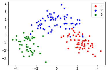
For a sample wine dataset taken from UCI ML Repository, initially, the dataset has 13 features, after the PCA algorithm the dimensionality reduces to 2 dimensions and the visualized result is the below image.

Manifold Learning:

Techniques from high-dimensionality statistics can also be used for dimensionality reduction. Using manifold learning and is used to create a low-dimensional projection of high-dimensional data. This is often used for data visualization.

T-distributed Stochastic Neighbor Embedding (t-SNE) is a manifold learning technique used to project higher dimensional data to lower dimensions (mostly 2 or 3 dimensions), for visualization. t-SNE is a neighborhood preserving embedding technique that best preserves the salient structure or relationships in the data in the lower dimension.

import pandas as pd
import seaborn as sns
from sklearn.preprocessing import StandardScaler
from sklearn.manifold import TSNE

data = pd.read_csv("Wine.csv")

X = data.iloc[:,:-1].values
y = data.iloc[:,-1].values

std = StandardScaler()
X_std = std.fit_transform(X)

tsne = TSNE(n_components=2, perplexity=50)
tsne_data = tsne.fit_transform(X_std)

sns.scatterplot(x=tsne_data[:,0], y=tsne_data[:,1], hue=y, palette=["red", "blue", "green"])
plt.show()

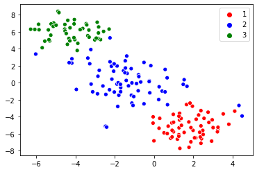
For a sample wine dataset taken from UCI ML Repository, initially, the dataset has 13 features, after applying the t-SNE algorithm the dimensionality reduces to 2 dimensions and the visualized result is the below image.

Auto Encoders:

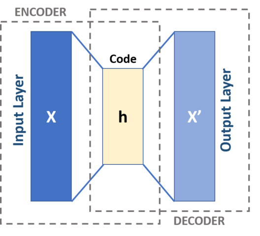
Auto Encoders is an artificial neural network model that performs dimensionality reduction. The autoencoder has 2 components, compression, and expansion. The initial dataset of shape (n rows, d dimensions) is passed to the autoencoder neural network model and is encoded to the lower dimension hidden layer. Then it tries to generate from the reduced encoding a representation as close as possible to its original input.

This article has been published from the source link without modifications to the text. Only the headline has been changed.

Source link