Understanding the data (error) generating processes

Statistics literature often makes reference to the data generating process (DGP): an idealized description of a real-world system responsible for producing observed data. This leads to a modeling approach focused on describing that system as opposed to blindly fitting observations to a common functional form.

As a trivial example, if one wished to model the height of a group of adults, they might suppose that the height of women and the height of men each is normally distributed with separate means and standard deviations. Then the overall distribution of population heights could be models as a mixture of samples from these two distributions.

However, DGPs are not only useful for modeling. Conceptualizing the DGP of our observations can also lead to more principled data validation if we broaden the scope of the DGP to include the subsequent manufacturing of the data not just the originating mechanism.

Unfortunately, consumers of analytical data may not always be familiar with the craft of data production (including data engineering, data modeling, and data management). Without an understanding of the general flow of data processing between collection and publication to a data warehouse, data consumers are less able to theorize about failure modes. Instead, similarly to blindly fitting models without an underlying theory, consumers may default to cursory checks of summary statistics without hypotheses for the kind of errors they are trying to detect or how these checks might help them.

This post explores the DGP of system-generated data and the common ways that these processes can introduce risks to data quality. As we discuss data validation, we will make reference to the six dimensions of data quality defined by DAMA: completeness, uniqueness, timeliness, validity, accuracy, and consistency. Along the way, we will explore how understanding how understanding key failure modes in the data production process can lead to more principled analytical data validation.

The Four DGPs for Data Management

To better theorize about data quality issues, it’s useful to think of four DGPs: the real-world DGP, the data collection/extraction DGP⁴, the data loading DGP, and the data transformation DGP.

For example, consider the role of each of these four DGPs for e-commerce data:

• Real-world DGP: Supply, demand, marketing, and a range of factors motivate a consumer to visit a website and make a purchase
• Data collection DGP: Parts of the website are instrumented to log certain customer actions. This log is then extracted from the different operational system (login platforms, payment platforms, account records) to be used for analysis
• Data loading DGP: Data recorded by different systems is moved to a data warehouse for further processing through some sort of manual, scheduled, or orchestrated job. These different systems may make data available at different frequencies.
• Data transformation DGP: To arrive at that final data presentation requires creating a data model to describe domain-specific attributes with key variables crafted with data transformations

Or, consider the role of each of these four DGPs for subway ridership data:

• Real-world DGP: Riders are motivated to use public transportation to commute, run errands, or visit friends. Different motivating factors may cause different weekly and annual seasonality
• Data collection DGP: To ride the subway, riders go to a station and enter and exit through turnstiles. The mechanical rotation of the turnstile caused by a rider passing through is recorded
• Data loading DGP: Data recorded at each turnstile is collected through a centralized computer system at the station. Once a week, each station uploads a flat file of this data to a data lake owned by the city’s Department of Transportation
• Data transformation DGP: Turnstiles from different companies may have different data formats. Transformation may include harmonizing disparate sources, coding system-generated codes (e.g. Station XYZ) to semantically meaningful names (e.g. Main Street Station), and publishing a final unified representation across stations and across time

In the next sections, we’ll explore how understanding key concepts about each of these DGPs can help build a consumers’ intuition on where to look for problems.

Data Collection

Data collection is necessarily the first step in data production, but the very goal of data collection: translating complex human concepts into tabular data records is fraught with error. Data collection is effectively dimensionality reduction, and just like statistical dimensionality reduction, it must sometimes sacrifice accuracy for clarity.

This tradeoff makes data collection vulnerable to one of the largest risks to data validity: not that the data itself is incorrect given its stated purpose but rather that users misconstrue the population or metrics it includes. Thus, understanding what systems are intending to capture, publish, and extract and how they chose to encode information for those observations is essential for data validation and subsequent analysis.

Data collection can happen in countless different ways: experimentation, surveys, observation, sensors, etc. In many business settings, data is often extracted from source systems whose primary purpose is to execute some sort of real-world process. Such systems may naturally collect data for operational purposes or may be instrumented to collect and log data as they are used. This production data is then often extracted from a source system to an alternative location such as a data warehouse for analysis.

What Counts

One of the tricky nuances of data collection is understanding what precisely is getting captured and logged in the first place.

Consider something as simple as a login system where users must enter their credentials, endure a Captcha-like verification process to prove that they are not a robot, and enter a multi-factor authentication code.

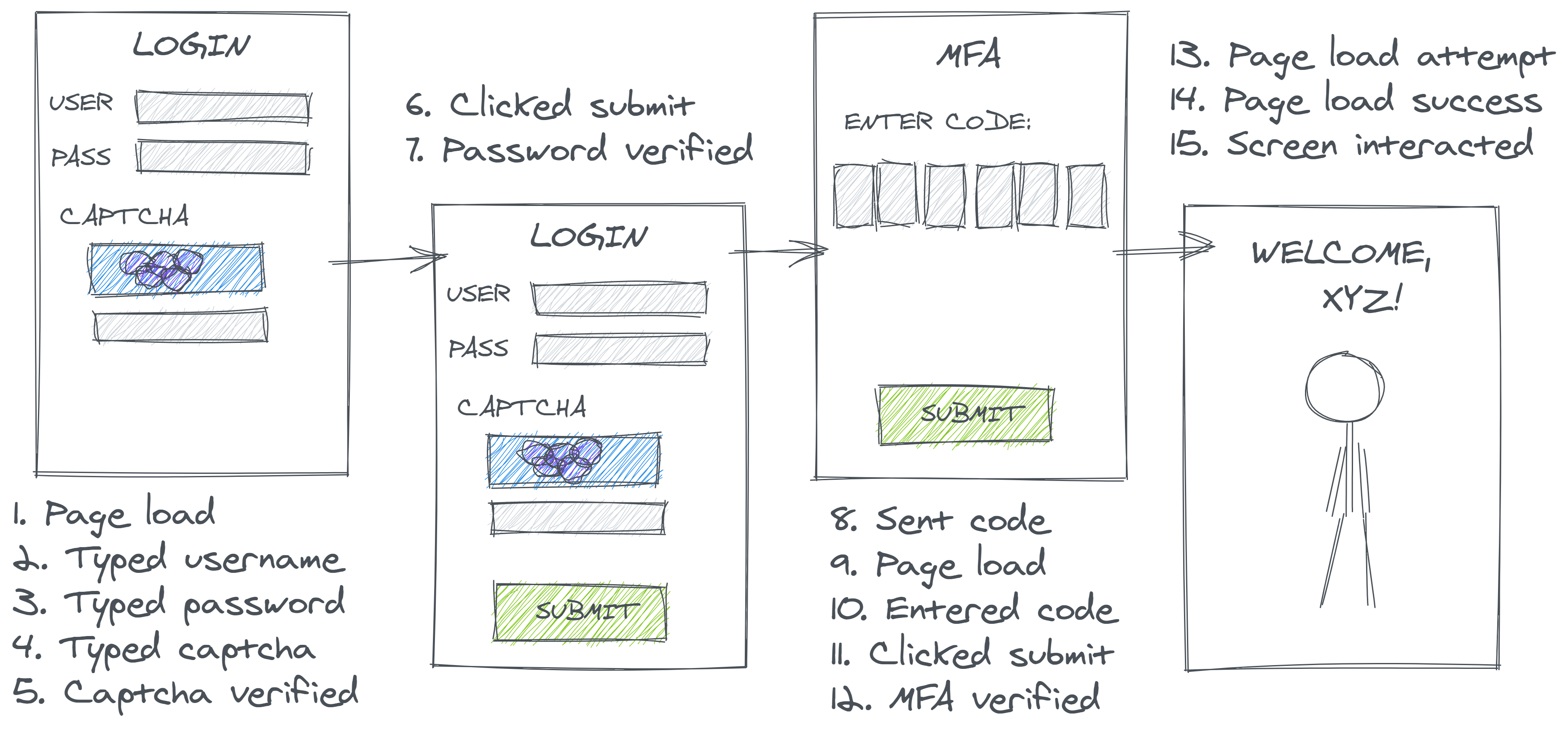
Which of these events gets collected and recorded has a significant impact on subsequent data processing. In a technical sense, no inclusion/exclusion decision here is incorrect, persay, but if the producers’ choices don’t match the consumers’ understandings, it can lead to misleading results.

For example, an analyst might seek out a logins table in order to calculate the rate of successful website logins. Reasonably enough, they might compute this rate as the sum of successful events over the total. Now, suppose two users attempt to login to their account, and ultimately, one succeeds in accessing their private information and the other doesn’t. The analyst would probably hope to compute and report a 50% login success rate. However, depending on how the data is represented, they could quite easily compute nearly any value from 0% to 100%.

• Per Attempt: If data is logged once per overall login attempt, successful attempts only trigger one event, but a user who forgot their password may try (and fail) to login multiple times. In the case illustrated above, that deflates the successful login rate to 25%.
• Per Event: If the logins table contains a row for every login-related event, each ‘success’ will trigger a large number of positive events and each ‘failure’ will trigger a negative event preceded by zero or more positive events. In the case illustrated below, this inflates our successful login rate to 86%.
• Per Conditional: If the collector decided to only look at downstream events, perhaps to circumvent record duplication, they might decide to create a record only to denote the success or failure of the final step in the login process (MFA). However, login attempts that failed an upstream step would not generate any record for this stage because they’ve already fallen out of the funnel. In this case, the computed rate could reach 100%
• Per Intermediate: Similarly, if the login was defined specifically as successful password verification, the computed rate could his 100% even if some users subsequently fail MFA

	Session	Attempt	Attempt	Outcome	Intermediate
Success	1	1	6	1	2
Total	2	4	7	1	2
Rate	50%	25%	86%	100%	100%

While humans have a shared intuition of what concepts like a user, session, or login are, the act of collecting data forces us to map that intuition onto an atomic event . Any misunderstanding in precisely what that definition is can have massive impact on the perceived data quality; “per event” data will appear heavily duplicated if it is assumed to be “per session” data.

In some cases, this could be obvious to detect. If the system outputs fields that are incredibly specific (e.g. with some hyperbole, imagine a step_in_the_login_process field with values taking any of the human-readable descriptions of the fifteen processes listed in the image above), but depending how this source is organized (e.g. in contrast to above, if we only have fields like sourceid and processid with unintuitive alphanumeric encoded values) and defined, it could be nearly impossible to understand the nuances without uncovering quality metadata or talking to a data producer.⁷

What Doesn’t Count

Along with thinking about what does count (or gets logged), it’s equally important to understand what systemically does not generate a record. Consider users who have the intent or desire to login (motivated by a real-world DGP) but cannot find the login page, or users who load the login page but never click a button because they know that they’ve forgotten their password and see no way to request it. Often, some of these corner cases may be some of the most critical and informative (e.g. here, demonstrating some major flaws in our UI). It’s hard to computationally validate what data doesn’t exist, so conceptual data validation is critical.

The Many Meanings of Null

Related to the presence and absence of full records is the presence or absence of individual fields. If records contain some but not all relevant information, they may be published with explicitly missing fields or the full record may not be published at all.

Understanding what the system implies by each explicitly missing data field is also critical for validation and analysis. Checks for data completeness usually include counting null values, but null data isn’t always incorrect. In fact, null data can be highly informative if we know what it means. Some meanings of null data might include:

• Field is not relevant: Perhaps our logins table reports the mobile phone operating system (iOS or Android) that was used to access the login page to track platform-specific issues. However, there is no valid value for this
• Relevant value is not known: Our logins table might also have an account_id field which attempts to match login attempts to known accounts/customers using different metadata like cookies or IP addresses. In theory, almost everyone trying to log in should have an account identifier, but our methods may not be good enough to identify them in all cases
• Relevant value is null: Of course, sometimes someone without an account at all might try to log in for some reason. In this case, the correct value for an account_id field truly is null
• Relevant value was recorded incorrectly: Sometimes systems have glitches. Without a doubt, every single login attempt should have a timestamp, but such a field could be null if this data was somehow lost or corrupted at the source

Similarly, different systems might or might not report out these nulls in different ways such as:

• True nulls: Literally the entry in the resulting dataset is null
• Null-like non-nulls: Blank values like an empty string ('') that contain a null amount of information but won’t be detected when counting null values
• Placeholder values: Meaningless values like an account_id of 00000000 for all unidentified accounts which preserve data validity (the expected structure) but have no intrinsic meaning
• Sentinel/shadow values: Abnormal values which attempt to indicate the reasons for null-ness such as an account_id of -1 when no browser cookies were found or -2 when cookies were found but did not help link to any specific customer record

Each of these encoding choices changes the definitions of appropriate completeness and validity for each field and, even more critically, impacts the expectations and assertions we should form for data accuracy. We can’t expect 100% completeness if nulls are a relevant value; we can’t check validity of ranges as easily if sentinel values are used with values that are outside the normal range (hopefully, or we have much bigger problems!) So, understanding how upstream systems should work is essential for assessing if they do work.

Data Loading

Checking that data contains expected and only expected records (that is, completeness, uniqueness, and timeliness) is one of the most common first steps in data validation. However, the superficially simple act of loading data into a data warehouse or updating data between tables can introduce a variety of risks to data completeness which require different strategies to detect. Data loading errors can result in data that is stale, missing, duplicate, inconsistently up-to-date across sources, or complete but for only a subset of the range you think.

While the data quality principles of completeness, uniqueness, and timeliness would suggest that records should exist once and only once, the reality of many haphazard data loading process means data may appear sometime between zero and a handful of times. Data loads can occur in many different ways. For example, they might be:

• manually executed
• scheduled (like a cron job)
• orchestrated (with a tool like Airflow or Prefect)

No approach is free from challenges. For example, scheduled jobs risk executing before an upstream process has completed (resulting in stale or missing data); poorly orchestrated jobs may be prevented from working due to one missing dependency or might allow multiple stream to get out of sync (resulting in multisource missing data). Regardless of the method, all approaches must be carefully configured to handle failures gracefully to avoid creating duplicates, and the frequency at which they are executed may cause partial loading issues if it is incompatible with the granularity of the source data.

Data Load Failure Modes

For example, suppose in the diagram below that each row of boxes represents one day of records in a table.

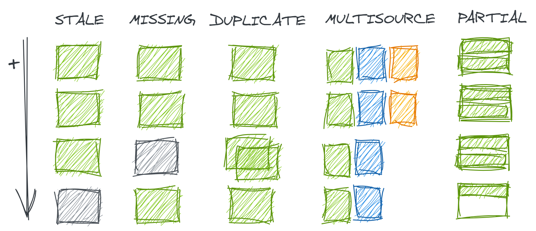
• Stale data occurs when the data is not as up-to-date as would be expected from is regular refresh cadence. This could happen if a manual step was skipped, a scheduled job was executed before the upstream source was available, or orchestrated data checks found errors and quarantined new records
• Missing data occurs when one data load fails but subsequent loads have succeeded
• Duplicate data occurs when one data load is executed multiple times
• Multisource missing data occurs when a table is loaded from multiple sources, and some have continued to update as expected while others have not
• Partial data occurs when a table is loaded correctly as intended by the producer but contains less data than expected by the consumer (e.g. a table loads ever 12 hours but because there is some data for a given date, the user assumes that all relevant records for that date have been loaded)

The differences in these failure modes become important when an analyst attempts to assess data completeness. One of the first approaches an analyst might consider is simply to check the min() and max() event dates in their table. However, this can only help detect stale data. To catch missing data, an analyst might instead attempt to count the number of distinct days represented in the data; to detect duplicate data, that analyst might need to count records by day and examine the pattern.

Metric	Stale	Missing	Duplicate	Multi	Partial
min(date) max(date)	1 3	1 4	1 4	1 4	1 4
count(distinct date)	3	3	4	4	4
count(1) by date	100 100 100 0	100 100 0 100	100 100 200 100	100 100 66 66	100 100 100 50
count(1) count(distinct PKs)	300 300	300 300	400 300	332 332	350 350

In a case like the toy example above where the correct number of rows per date is highly predictable and the number of dates is small, such eyeballing is feasible; however when the expected number of records varies day-to-day or time series are long, this approach becomes subjective, error-prone, and intractable. Additionally, it still might be hard to catch errors in mutli-source data or partial loads if the lower number of records was still within the bounds of reasonable deviation for a series. These last two types deserve further exploration.

Multi-Source

A more effective strategy for assessing data completeness requires a better understanding of how data is being collected and loaded. In the case of multi-source data, one single source stopping loading may not be a big enough change to disrupt aggregate counts but could still jeopardize meaningful analysis. It would be more useful to conduct completeness checks by subgroup to identify these discrepancies.

But not any subgroup will do; the subgroup must correspond to the various data sources. For example, suppose we run an e-commerce store and wish to look at sales from the past month by category. Naturally, we might think to check the completeness of the data by category. But what if sales data is sourced from three separate locations: our Shopify site (80%), our Amazon Storefront (15%), and phone sales (5%). Unless we explicitly check completeness by channel (a dimension we don’t particularly care about for our analysis), it would be easy to miss if our data source for phone sales has stopped working or loads at a different frequency.

Another interesting aspect of multi-source data, is multiple sources can contribute either to different rows/records or different columns/variables. Table-level frequency counts won’t help us in the latter case since other sources might create the right total number of records but result in some specific fields in those records being missing or inaccurate.

Partial Loads

Partial loads really are not data errors at all, but are still important to detect since they can jeopardize an analysis. A common scenario might occur if a job loads new data every 12 hours (say, data from the morning and afternoon of day n-1 loads on day n at 12AM and 12PM, respectively). An analyst retrieving data at 11AM may be concerned to see an approximate ~50% drop in sales in the past day, despite confirming that their data looks to be “complete” since the maximum record date is, in fact, day n-1.

Delayed or Transient Records

The interaction between choices made in the data collection and data loading phases can introduce their own sets of problems.

Consider an orders table for an e-commerce company that analysts may use to track customer orders. It might contain one record per order_id x event (placement, processing, shipment), one record per order placed, one record per order shipping, or one record per order with a status field that changes over time to denote the order’s current stage of life.

Any of these modeling choices seem reasonable and the difference between them might appear immaterial. But consider the collection choice to record and report shipped events. Perhaps this might be operationally easier if shipment come from one source system whereas orders could come from many. However, an interesting thing about shipments is that they are often lagged in a variable way from the order date.

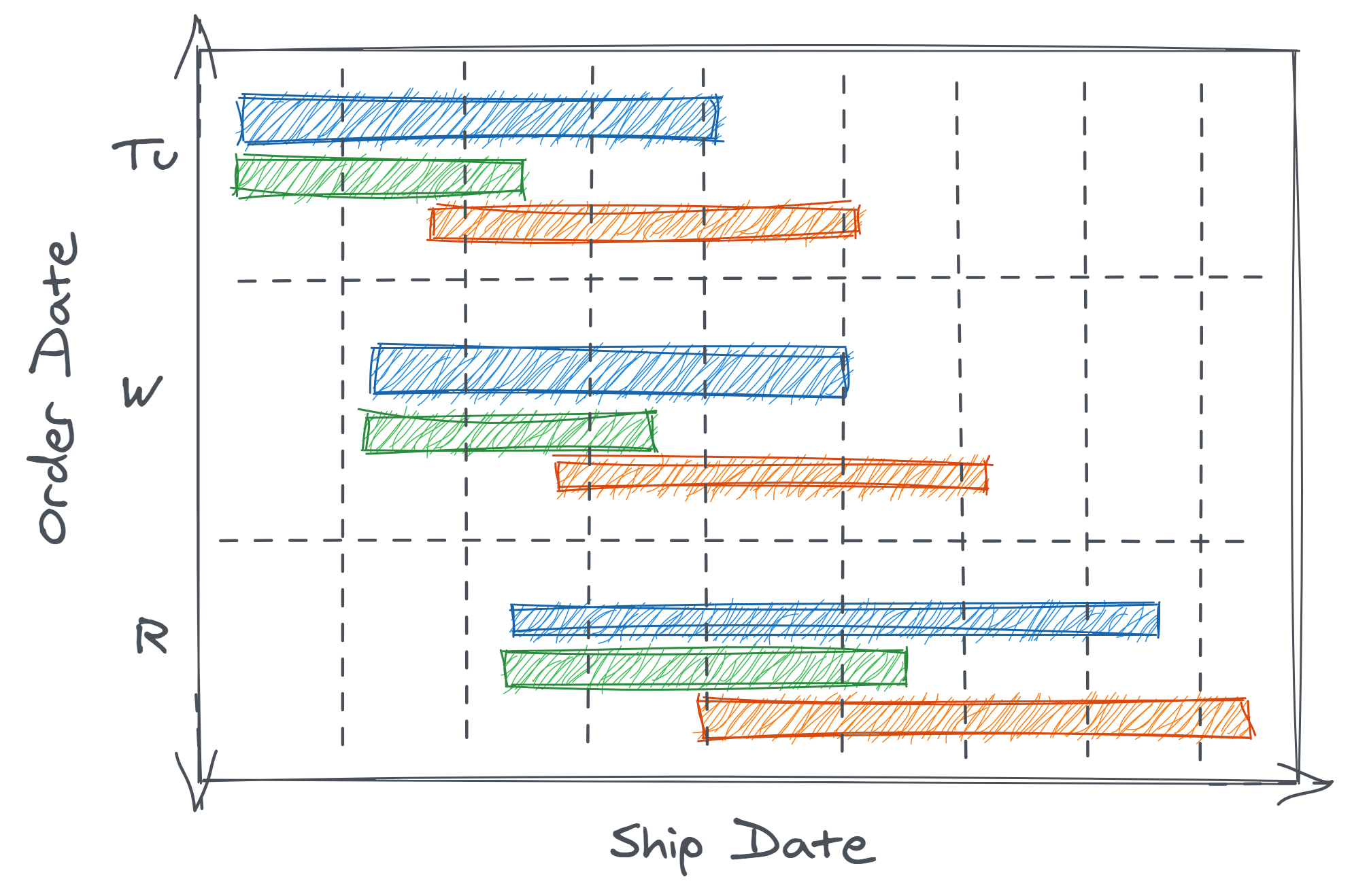
Suppose the e-commerce company in question offers three shipping speeds at checkout. The chart below shows the range of possible shipment dates based on the order dates for the three different speeds (shown in different bars/colors). How might this effect our perceived data quality?

• Order data could appear stale or not timely since orders with a given order_date would only load days later once shipped
• Similar to missing or multisource data, the data range in the table could lead to deceptive and incomplete data validation because some orders from a later order date might ship (and thus be logged) before all orders from a previous order date
• Put another way, we could have multiple order dates demonstrating partial data loads
• These features of the data might behave inconsistently across time due to seasonality (e.g. no shipping on weekends or federal holidays), so heuristics developed to clean the data based on a small number of observations could fail
• From an analytical perspective, orders with faster shipping would be disproportionately overrepresented in the “tail” (most recent) data. If shipping category correlated with other characteristics like total order spend, this could create an artificial trend in the data

Once again, understanding that data is collected at point of shipment and reasoning how shipment timing varies and impacts loading is necessary for successful validation.

Data Transformation

Finally, once the data is roughly where we want it, it likely undergoes many transformations to translate all of the system-generated fields we discussed in data collection into semantically-relevant dimensions for analytical consumers. Of course, the types of transformations that could be done are innumerable with far more variation than data loading. So, we’ll just look at a few examples of common failure patterns.

Pre-Aggregation

Data transformations may include aggregating data up to higher levels of granularity for easier analysis. For example, a transformation might add up item-level purchase data to make it easier for an analyst to look at spend per order of a specific user.

Data transformations not only transform our data, but they also transform how the dimensions of data quality manifest. If data with some of the completeness or uniqueness issues we discussed with data loading is pre-aggregated, these problems can turn into problems of accuracy. For example, the duplicate or partial data loads that we discussed when aggregated could suggest inaccurately high or low quantities respectively.

Field Encoding

When we assess data consistency across tables,

Categorical fields in a data set might be created in any number of ways including:

• Directly taken from the source
• Coded in a transformation script
• Transformed with logic in a shared user-defined function ( UDFs) or macro
• Joined from a shared look-up table

Each approach has different implications on data consistency and usability.

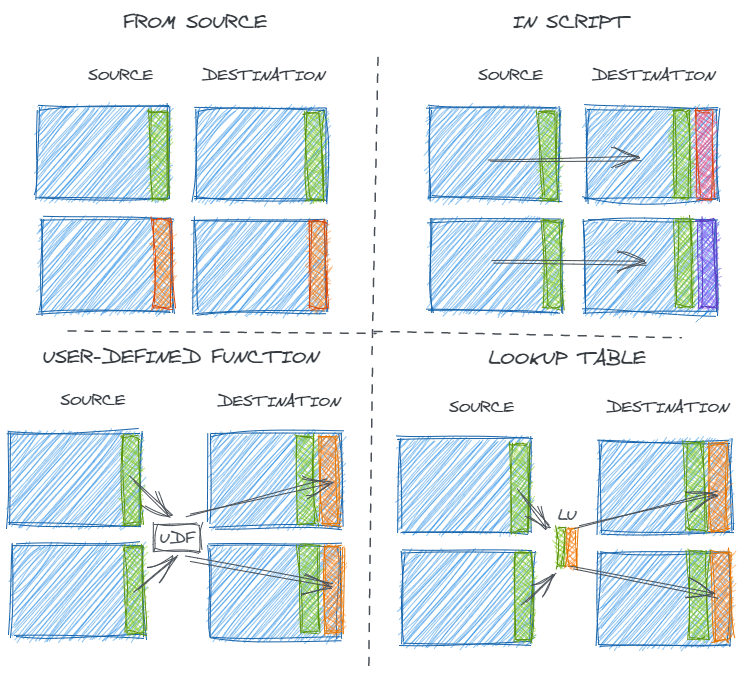
Using fields from the source simply is what it is – there’s no subjectivity or room for manual human error. If multiple tables come from the same source, it’s likely but not guaranteed that they will be encoded in the same way.

Coding transformations in the ELT process is easy for data producers. There’s no need to coordinate across multiple processes or use cases, and the transformation can be immediately modified when needed. However, that same lack of coordination can lead to different results for fields that should be the same.

Alternatively, macros, UDFs, and look-up tables provided centralized ways to map source data inputs to desired analytical data outputs in a systemic and consistent way. Of course, centralization has its own challenges. If something in the source data changes, the process of updating a centralized UDF or look-up table may be slowed down by the need to seek consensus and collaborate. So, data is more consistent but potentially less accurate.

Regardless, such engineered values require scrutiny – paticularly if they are being used as a key to join multiple tables – and the distinct values in them should be carefully examined.

Updating Transformations

Of course, data consistency is not only a problem across different data sources but within one data source. Regardless of the method of field encoding used in the previous step, the intersection of data loading and data transformation strategies can introduce data consistency errors over time.

Often, for computation efficiency, analytical tables are loaded using an incremental loading strategy. This means that only new records (determined by time period, a set of unique keys, or other criteria) from the upstream source are loaded to the downstream table. This is in contrast to a full refresh where the entire downstream table is recreated on each update.

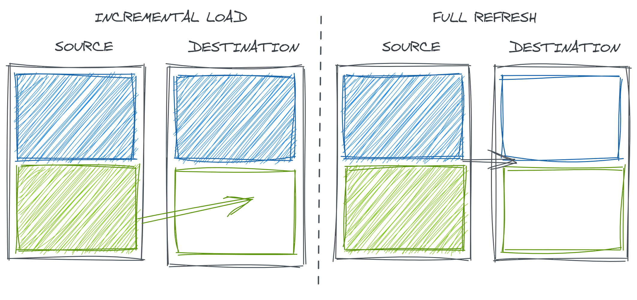
Incremental loads have many advantages. Rebuilding tables in entirety can be very time consuming and computationally expensive. In particular, in non-cloud data warehouses that are not able to scale computing power on demand, this sort of heavy duty processing job can noticeably drain resources from other queries that are trying to run in the database. Additionally, if the upstream staging data is ephemeral, fully rebuilding the table could mean failing to retain history.

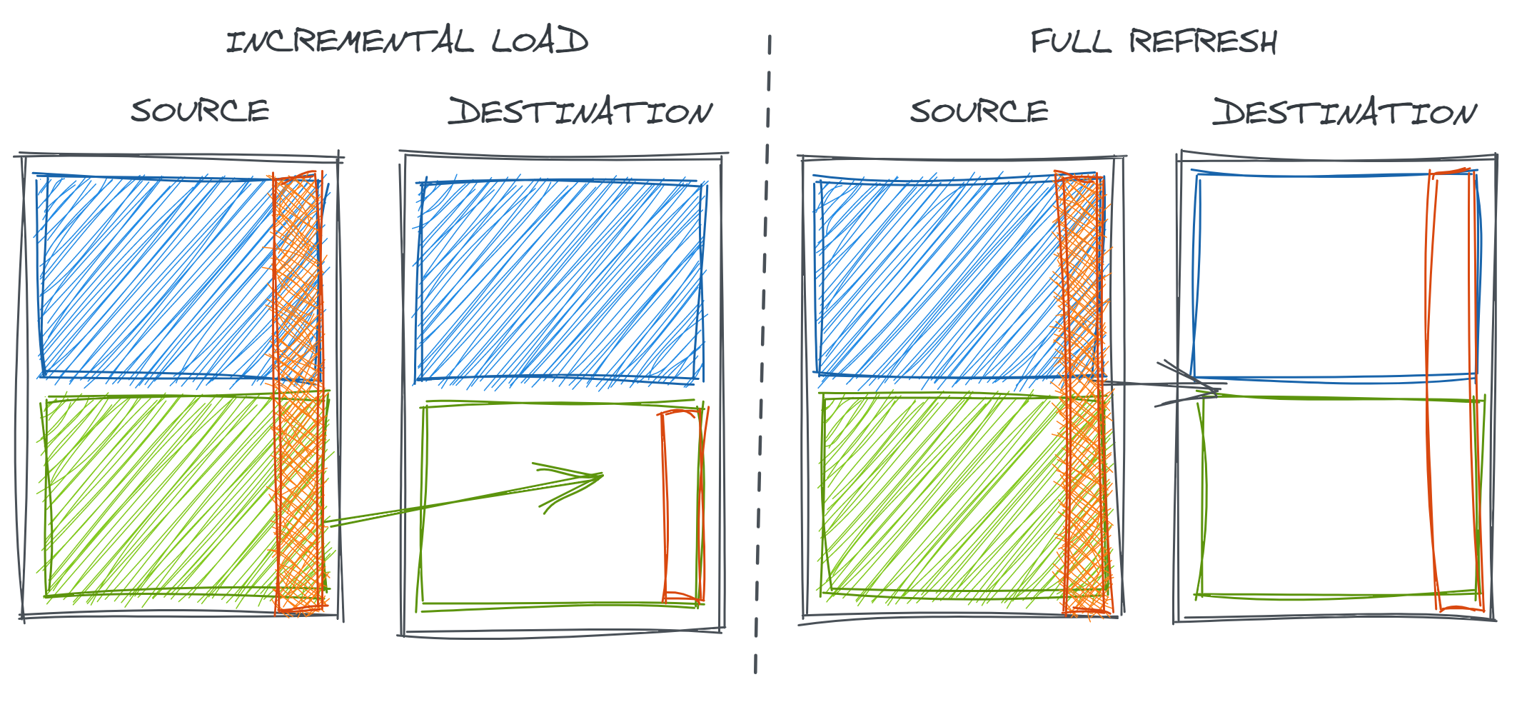
However, in the case that our data transformations change, incremental loads may introduce inconsistency in our data overtime as only new records are created and inserted with the new logic.

This is also a problem more broadly if some short-term error is discovered either with data loading or transformation in historical data. Incremental strategies may not always update to include the corrected version of the data.

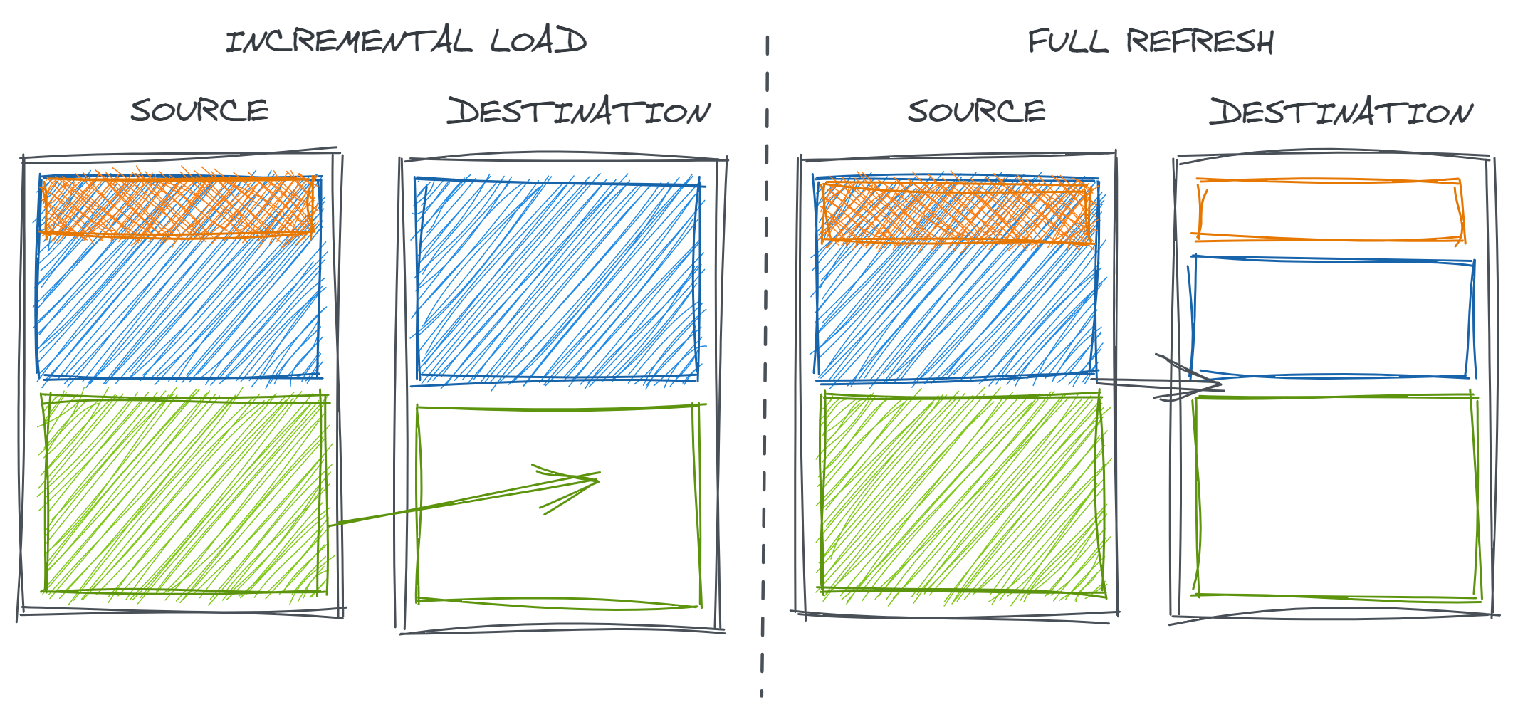
Regardless, this underscores the need to validate entire datasets and to re-validate when repulling data.

Conclusion

In statistical modeling, the goal of considering the data generating process is not to understand an encode every single nuance of the complete DGP. After all, if all of that were known, we wouldn’t need a model: we could simulate the universe.

Similarly for data validation, data consumers cannot know everything about the data production DGP without taking over the data production process in its entirety. But understanding some of the key failure modes faced by data producers can support data validation by helping consumers develop more realistic theories and expectations for the ways data may ‘break’ and how to refine strategies for detection them.

This article has been published from the source link without modifications to the text. Only the headline has been changed.

Source link