Training Neural Networks through Regularization Techniques

Regularization is a set of strategies used in Machine Learning to reduce the generalization error. Most models, after training, perform very well on a specific subset of the overall population but fail to generalize well. This is also known as overfitting. Regularization strategies aim to reduce overfitting and keep, at the same time, the training error as low as possible.

TL;DR

In this article, we will present a review of the most popular regularization techniques used when training Deep Neural Networks. We will categorize these techniques on bigger families based on their similarities.

Why regularization?

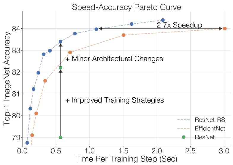
You have probably heard of the famous ResNet CNN architecture. ResNets were originally proposed in 2015. A recent paper called “Revisiting ResNets: Improved Training and Scaling Strategies” applied modern regularization methods and achieved more than 3% test set accuracy on Imagenet.

If the test set consists of 100K images, this means that 3K more images were classified correctly!

Awesome, isn’t it?

Now, let’s cut to the chase.

What is regularization?

According to Ian Goodfellow, Yoshua Bengio and Aaron Courville in their Deep Learning Book:

“In the context of deep learning, most regularization strategies are based on regularizing estimators. Regularization of an estimator works by trading increased bias for reduced variance. An effective regularizer is one that makes a profitabletrade, reducing variance significantly while not overly increasing the bias.”

In simple terms, regularization results in simpler models. And as the Occam’s razor principle argues: the simplest models are the most likely to perform better. Actually, we constrain the model to a smaller set of possible solutions by introducing different techniques.

To get a better insight you need to understand the famous bias-variance tradeoff.

The bias-variance tradeoff: overfitting and underfitting

First, let’s clarify that bias-variance tradeoff and overfitting-underfitting are equivalent.

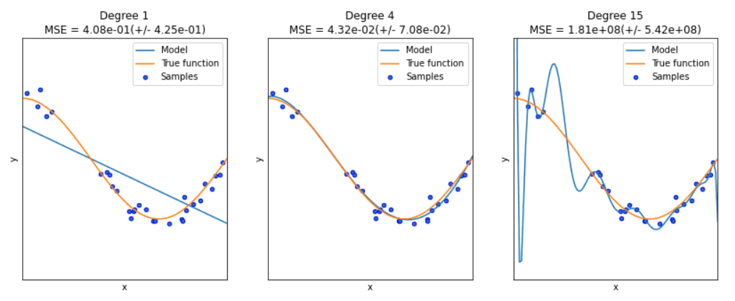
Underfitting and overfitting. Source: datascience.foundation/

The bias error is an error from wrong assumptions in the learning algorithm. High bias can cause an algorithm to miss the relevant relations between features and target outputs. This is called underfitting.

The variance is an error from sensitivity to small fluctuations in the training set. High variance may result in modeling the random noise in the training data. This is called overfitting.

The bias-variance tradeoff is a term to describe the fact that we can reduce the variance by increasing the bias. Good regularization techniques strive to simultaneously minimize the two sources of error. Hence, achieving better generalization.

As a side material, I highly recommend the DeepLearning.Ai course: Improving Deep Neural Networks: Hyperparameter Tuning, Regularization and Optimization

How to introduce regularization in deep learning models

Modify the loss function: add regularization terms

The most common family of approaches used before the Deep Learning era in estimators such as linear and logistic regression, are parameters norm penalties. Here we add a parameter norm penalty $\Omega (\theta )$ to the loss function $J(\theta ;X,y)$:

where $\theta$ denotes the trainable parameters, $X$ the input, and $y$ and target labels. $a$ is a hyperparameter that weights the contribution of the norm penalty, hence the effect of the regularization.

Ok, the math looks good. But why exactly does this work? Let’s look at the two most popular methods to make that crystal clear. L2 and L1.

L2 regularization

L2 regularization, also known as weight decay or ridge regression, adds a norm penalty in the form of \Omega(\theta) = \frac{1}{2}||w||^2_2Ω(θ)=21​∣∣w∣∣22​ . The loss function has been transformed to:

If we compute the gradients we have:

For a single training step and a learning rate $\lambda$, this can be written as:

The equation effectively shows us that each weight of the weight vector will be reduced by a constant factor on each training step.

Note here that we replaced $\theta$ with $w$. This was due to the fact that usually we regularize only the actual weights of the network and not the biases $b$.

If we look at it from the viewpoint of the entire training here is what happens:

The L2 regularizer will have a big impact on the directions of the weight vector that don’t “contribute” much to the loss function. On the other hand, it will have a relatively small effect on the directions that contribute to the loss function. As a result, we reduce the variance of our model, which makes it easier to generalize on unseen data.

L1 regularization

L1 regularization chooses a norm penalty of \Omega(\theta) = ||w||_1 = \sum_i |w_i|Ω(θ)=∣∣w∣∣1​=∑i​∣wi​∣. In this case, the gradient of the loss function becomes:

As we can see, the regularization term does not scale linearly, contrary to L2 regularization, but it’s a constant factor with an alternating sign. How does this affect the overall training?

The L1 regularizer introduces sparsity in the weights by forcing more weights to be zero instead of reducing the average magnitude of all weights ( as the L2 regularizer does). In other words, L1 suggests that some features should be discarded whatsoever from the training process.

Elastic net

Elastic net is a method that linearly combines L1 and L2 regularization with the goal to acquire the best of both worlds . More specifically the penalty term is as follows:

Elastic Net regularization reduces the effect of certain features, as L1 does, but at the same time, it does not eliminate them. So it combines feature elimination from L1 and feature coefficient reduction from the L2.

Entropy Regularization

Entropy regularization is another norm penalty method that applies to probabilistic models. It has also been used in different Reinforcement Learning techniques such as A3C and policy optimization techniques. Similarly to the previous methods, we add a penalty term to the loss function.

If we assume that the model outputs a probability distribution $p(x)$, then the penalty term will be denoted as:

The term “Entropy” has been taken from information theory and represents the average level of “information” inherent in the variable’s possible outcomes. An equivalent definition of entropy is the expected value of the information of a variable.

One very simple explanation of why it works is that it forces the probability distribution towards the uniform distribution to reduce variance.

In the context of Reinforcement Learning, one can say that the entropy term added to the loss, promotes action diversity and allows better exploration of the environment. For more information on policy gradients and A3C, check our previous articles: Unravel Policy Gradients and REINFORCE and The idea behind Actor-Critics and how A2C and A3C improve them.

Label smoothing

Noise injection is one of the most powerful regularization strategies. By adding randomness, we can reduce the variance of the models and lower the generalization error. The question is how and where do we inject noise?

Label smoothing is a way of adding noise at the output targets, aka labels. Let’s assume that we have a classification problem. In most of them, we use a form of cross-entropy loss such as -\sum_{c=1}^M y_{o,c}\log(p_{o,c})−∑c=1M​yo,c​log(po,c​) and softmax to output the final probabilities.

The target vector has the form of [0, 1 , 0 , 0]. Because of the way softmax is formulated: ( \sigma (\mathbf {z} )_{i}={\frac {e^{z_{i}}}{\sum _{j=1}^{K}e^{z_{j}}}}σ(z)i​=∑j=1K​ezj​ezi​​), it can never achieve an output of 1 or 0. The best he can do is something like [0.0003, 0.999, 0.0003, 0.0003]. As a result, the model will continue to be trained, pushing the output values as high and as low as possible. The model will never converge. That, of course, will cause overfitting.

To address that, label smoothing replaces the hard 0 and 1 targets by a small margin. Specifically, 0 are replaced with \frac{\epsilon}{ k-1}k−1ϵ​ and 1 with $1-ϵ$, where $k$ is the number of classes.

Dropout

Another strategy to regularize deep neural networks is dropout. Dropout falls into noise injection techniques and can be seen as noise injection into the hidden units of the network.

In practice, during training, some number of layer outputs are randomly ignored (dropped out) with probability $p$.

During test time, all units are present, but they have been scaled down by $p$. This is happening because after dropout, the next layers will receive lower values. In the test phase though, we are keeping all units so the values will be a lot higher than expected. That’s why we need to scale them down.

By using dropout, the same layer will alter its connectivity and will search for alternative paths to convey the information in the next layer. As a result, each update to a layer during training is performed with a different “view” of the configured layer. Conceptually, it approximates training a large number of neural networks with different architectures in parallel.

“Dropping” values means temporarily removing them from the network for the current forward pass, along with all its incoming and outgoing connections. Dropout has the effect of making the training process noisy. The choice of the probability $p$ depends on the architecture.

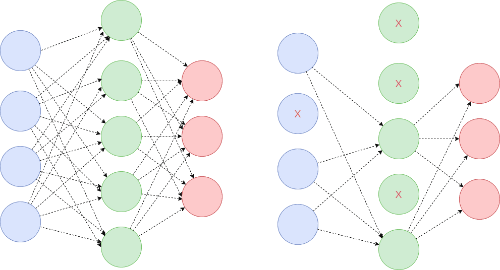
This conceptualization suggests that perhaps dropout breaks up situations where network layers co-adapt to correct mistakes from prior layers, making the model more robust. It increases the sparsity of the network and in general, encourages sparse representations! Sparsity can be added to any model with hidden units and is a powerful tool in our regularization arsenal.

Other Dropout variations

There are many more variations of Dropout that have been proposed over the years. To keep this article relatively digestible, I won’t go into many details for each one. But I will briefly mention a few of them. Feel free to check out paperswithcode.com for more details on each one, alongside the original paper and code.

1. Inverted dropout also randomly drops some units with a probability $p$. The difference with traditional dropout is: During training, it also scales the activations by the inverse of the keep probability $1-p$. The reason behind this is: to prevent the activations from becoming too large thus the need to modify the network during the testing phase. The end result will be similar to the traditional dropout.
2. Gaussian dropout: instead of dropping units during training, is injecting noise to the weights of each unit. The noise is, more often than not ,Gaussian. This results in:
   1. A reduction in the computational effort during testing time.
   2. No weight scaling is required.
   3. Faster training overall
3. DropConnect follows a slightly different approach. Instead of zeroing out random activations (units), it zeros random weights during each forward pass. The weights are dropped with a probability of $1-p$. This essentially transforms a fully connected layer to a sparsely connected layer. Mathematically we can represent DropConnect as: $r=a\left((M\ast W)v\right)$ where $r$ is the layers’ output, $v$ the input, $W$ the weights and $M$ a binary matrix. $M$ is a mask that instantiates a different connectivity pattern from each data sample. Usually, the mask is derived from each training example. DropConnect can be seen as a generalization of Dropout to the full-connection structure of a layer.
4. Variational Dropout: we use the same dropout mask on each timestep. This means that we will drop the same network units each time. This was initially introduced for Recurrent Neural Networks and it follows the same principles as variational inference.
5. Attention Dropout: popular over the past years because of the rapid advancements of attention-based models like Transformers. As you may have guessed, we randomly dropped certain attention units with a probability $p$.
6. Adaptive Dropout: a technique that extends dropout by allowing the dropout probability to be different for different units. The intuition is that there may be hidden units that can individually make confident predictions for the presence or absence of an important feature or combination of features.
7. Embedding Dropout: a strategy that performs dropout on the embedding matrix and is used for a full forward and backward pass.
8. DropBlock: is used in Convolutional Neural networks and it discards all units in a continuous region of the feature map.

Stochastic Depth

Stochastic depth goes a step further. It drops entire network blocks while keeping the model intact during testing. The most popular application is in large ResNets where we bypass certain blocks through their skip connections.

In particular, Stochastic depth (Huang et al., 2016) drops out each layer in the network that has residual connections around it. It does so with a specified probability $p$ that is a function of the layer depth.

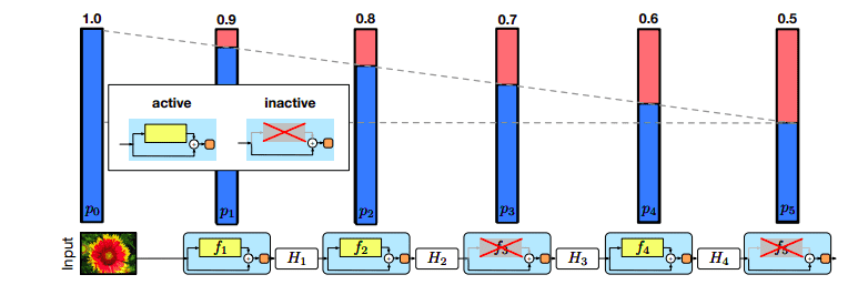
Source: Deep Networks with Stochastic Depth

Mathematically we can express this as:

where $b$ is a Bernoulli random variable that shows if a block is active or inactive. If $b=0$ the block will be inactive and if $b=1$ active.

Early stopping

Early stopping is one of the most commonly used strategies because it is very simple and quite effective. It refers to the process of stopping the training when the training error is no longer decreasing but the validation error is starting to rise.

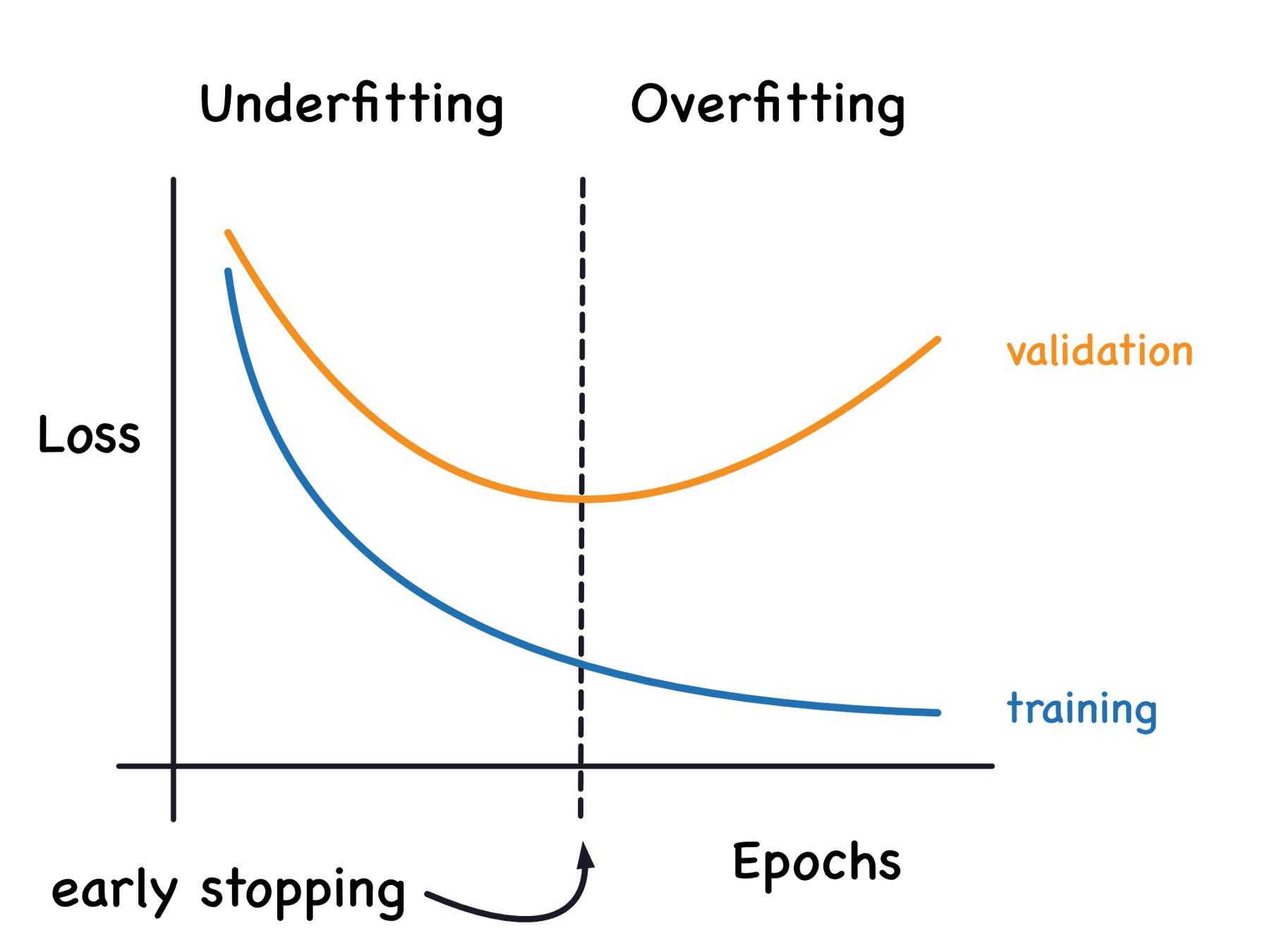
Source: kaggle.com

This implies that we store the trainable parameters periodically and track the validation error. After the training stopped, we return the trainable parameters to the exact point where the validation error started to rise, instead of the last ones.

A different way to think of early stopping is as a very efficient hyperparameter selection algorithm, which sets the number of epochs to the absolute best. It essentially restricts the optimization procedure to a small volume of the trainable parameters space close to the initial parameters.

It can also be proven that in the case of a simple linear model with a quadratic error function and simple gradient descent, early stopping is equivalent to L2 regularization.

Parameter sharing

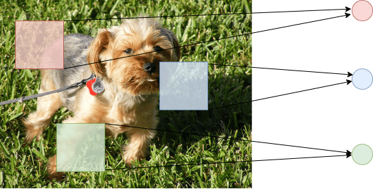
Parameter sharing follows a different approach. Instead of penalizing model parameters, it forces a group of parameters to be equal. This can be seen as a way to apply our previous domain knowledge to the training process. Various approaches have been proposed over the years but the most popular one is by far Convolutional Neural Networks.

Convolutional Neural Networks take advantage of the spatial structure of images by sharing parameters across different locations in the input. Since each kernel is convoluted with different blocks of the input image, the weight is shared among the blocks instead of having separate ones.

Batch normalization

Batch normalization (BN) can also be used as a form of regularization. Batch normalization fixes the means and variances of the input by bringing the feature in the same range. More specifically, we concentrate the features in a compact Gaussian-like space.

Visually this can be represented as:

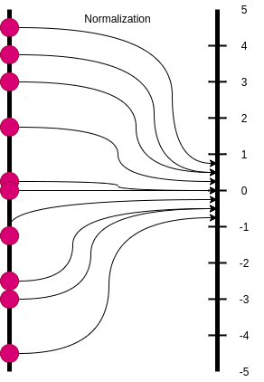
While mathematically we have:

Where $\gamma$ and $\beta$ are learnable parameters.

Batch normalization can implicitly regularize the model and in many cases, it is preferred over Dropout.

Why?

Here unfortunately there is not a clear answer. Just empirical observations.

One can think of batch normalization as a similar process with dropout because it essentially injects noise. Instead of multiplying each hidden unit with a random value, it multiplies them with the deviation of all the hidden units in the minibatch. It also subtracts a random value (the mean of the minibatch) from each hidden unit at each step.

Both of these “noises” will make the model more robust and reduce its variance. A great overview of why BN acts as a regularizer can be found in Luo et al, 2019.

Data augmentation

Data augmentation is the final strategy that we need to mention. Although not strictly a regularization method, it sure has its place here.

Data augmentation refers to the process of generating new training examples to our dataset. More training data means lower model’s variance, a.k.a lower generalization error. Simple as that. It can also be seen as a form of noise injection in the training dataset.

Data augmentation can be achieved in many different ways. Let’s explore some of them.

1. Basic Data Manipulations: The first simple thing to do is to perform geometric transformations on data. Most notably, if we’re talking about images we have solutions such as: Image flipping, cropping, rotations, translations, image color modification, image mixing etc. Cutout is a commonly used idea where we remove certain image regions. Another idea, called Mixup, is the process of blending two images from the dataset into one image.
2. Feature Space Augmentation : Instead of transforming data in the input space as above, we can apply transformations on the feature space. For example, an autoencoder might be used to extract the latent representation. Noise can then be added in the latent representation which results in a transformation of the original data point.
3. GAN-based Augmentation: Generative Adversarial Networks have been proven to work extremely well on data generation so they are a natural choice for data augmentation.
4. Meta-Learning: In meta-learning, we use neural networks to optimize other neural networks by tuning their hyperparameters, improving their layout, and more. A similar approach can also be applied in data augmentation. In simple terms, we use a classification network to tune an augmentation network into generating better images. Example: We feed random images to an Augmentation Network (most likely a GAN), which will generate augmented images. Both the augmented image and the original are passed into a second network, which compares them and tells us how good the augmented image is. After repeating the process the augmentation network becomes better and better at producing new images.

Conclusion

Regularization is an integral part of training Deep Neural Networks. In my mind , all the aforementioned strategies fall into two different high-level categories. They either penalize the trainable parameters or they inject noise somewhere along the training lifecycle. Whether this is on the training data, the network architecture, the trainable parameters or the target labels.

This article has been published from the source link without modifications to the text. Only the headline has been changed.

Source link