In recent — as well as not-so-recent — years, many different unsupervised learning methods have been proposed. Unsupervised learning methods summarize data or transform it such that some desirable properties are enforced. These properties are often easily achieved analytically but are harder to enforce when working in a stochastic optimization (e.g. neural network) framework.

Inductive biases

Before a model is created or a method is defined, some groundwork needs to be laid. What assumptions do we make about the data or the model? How do we know that the model we end up with is good and what do we exactly mean by good?

Every model comes prepackaged with its set of inductive biases. Support vector machines aim at maximizing the margin between the classes, shorter decision trees are preferred over longer ones, e.t.c. Beyond machine learning, a famous inductive bias is Occam’s razor in the sciences (The simplest solution is most likely the right one.) as well as its engineering cousin, the KISS principle (Keep it simple, stupid!).

Note: This is called a regularization strategy rather than an inductive bias in the Deep Learning book, but I associate “regularization” with something used to mitigate overfitting. Although we’re not doing inference here, I choose to call a generic prior used to guide learning an inductive bias. Ferenc Huszár uses this nomenclature in his blog and I will call it like that for now as well.

Motivating a couple of inductive biases

A way that we might want to describe things is in terms of independent features. A feature is just an additional property of the data which you can suss out from the data directly. For example, the number of black pixels in a photograph, your material advantage in a game of chess and so on. For the features to be (statistically) independent means that knowledge of one doesn’t tell you anything about the other.

Why would we want features to be independent? It’s easy to overlook the importance of independent features, as it’s so natural to think of the world as composed of independent parts. I like this scenario:

As an example, imagine the following: a language called Grue, with the following 2 concepts (i.e. words): “grue”: green by day, but blue by night, and “bleen”: blue by day, but green by night. Now, using the Grue language, describing a blue-eyed person would be quite complicated, as you’d have to say: this person has eyes that are grue at night, but bleen during daylight.
— stensool

We can see that the concepts of colors and time are not independent in the Grue language (something can’t be “grue” and “bleen” simultaneously) and that describing the world using dependent terms introduces a lot of unnecessary complications.

Another way we might want to describe our world is in terms of slow features. A feature being slow isn’t a knock on it, but rather underlining that it changes slowly with time. It’s a concrete way of encouraging the model to determine what elements are slowly changing, even though they are made up of fast-changing components. For example, imagine a film scene where the camera is zooming in gently on a face. Even though we perceive that nothing much is happening (since the perceptual features are changing only very slowly), the values on the pixel-level are changing very rapidly.

Let’s start slow

Slow features can be found with Slow Feature Analysis (SFA). Just to iterate, this isn’t a slow “feature analysis” but rather a method of finding slowly varying features of the data. These slow features are found by solving the optimization problem:

In plain English, we want to find terms that change as slowly as possible over time to describe what we observe. The constraints (2) — (4) enforce on them zero mean, unit variance and de-correlation. This helps us avoid degenerate solutions (any constant function trivially solves (1)), as well as making sure that we don’t end up with redundant features.

In practice, the expectations are replaced with sample values and we minimize the empirical risk. SFA solves this analytically along these lines:

1. Apply a non-linear function to the original data.
2. Sphere the data to fulfill (2)-(4)
3. Calculate the time derivatives of the sphered data
4. Find the directions of the least variation of the sphered data using PCA.
5. Get the slow features by projecting the sphered data onto the eigenvectors corresponding to the lowest eigenvalues

This method has been shown to be an accurate model of many aspects of our own visual system. A limitation of this approach is that the non-linearity needs to be hand-picked, which raises the question: would learning the whole process in an end-to-end manner be beneficial for extracting even slower, more meaningful features?

This is exactly what we did in our work: Gradient-Based Training of Slow Feature Analysis and Spectral Embeddings (To be presented in ACML 2019). We trained a deep neural network to solve the SFA optimization problem for videos of rotating objects. This can be done simply by training the network using (1) as the loss function, but the constraints need to be enforced via network architecture.

A few words on sphering

A data set X of features is said to be sphered if its covariance matrix is equal to the identity matrix, that is, if each feature is uncorrelated and with a variance of 1. The data can be transformed by multiplying it with a whitening matrix W such that WX = Y has unit diagonal covariance.

How could we enforce this in neural networks? A naive approach would be to add a sort of regularizing term to the loss function, constraining the output’s covariance matrix to be close to the identity matrix. This will introduce a trade-off between minimizing the objective function and enforcing the constraints, whereas their enforcement is non-negotiable. To this end, a differentiable sphering layer for Keras was created for our work. With the sphering performed in the second-to-last layer, all there is to be done is maximizing the slowness of the sphered signals.

Differentiable sphering

Now, the whitening matrix can be found analytically in a variety of ways, for example with PCA whitening. If we have zero-mean data with a covariance matrix Σ, we can perform an eigendecomposition and get Σ=UΛUᵀ (where Σ’s eigenvectors are in U with the corresponding eigenvalues arranged on Λ’s diagonal). This gives us our ingredients for our whitening matrix W = U (1/√D)Uᵀ. This can be done in a differentiable manner using power iterations, as the following iterative formula

will converge to the largest eigenvector of C. A hundred (computationally fast) iterations are sufficient and the eigenvector is subtracted from C

Graphical SFA

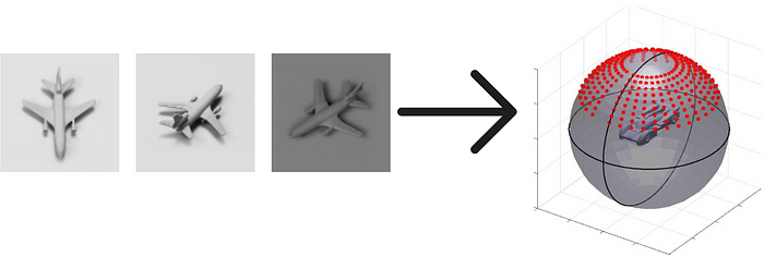
Since we have all our ingredients to deeply learn SFA, we can take it a step further. Instead of just minimizing the distance between representations of data points that are adjacent in time, we can work with a general similarity function and urge the representations to be similar for a priori known similar data points. For example, consider the NORB data set:

The globular visualization shows how the camera angles connect the different data points. If we were to connect each data point with their 4-neighbors (up, down, left, right) then we can minimize the loss function

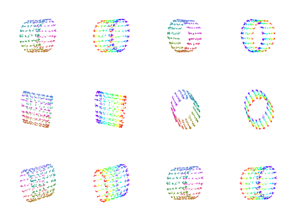
And get an essentially perfect, spherical embedding of the data:

Note that unlike methods such as Laplacian eigenmaps, this works on out-of-sample points!

Independent features

Remember that random variables A and B are independent if P(A∩B) = P(A)·P(B). The most famous algorithm for learning independent features of the data is Independent Component Analysis (ICA).

In ICA, the assumption is that our data X is a linear mixture of statistically independent sources S, i.e. X = WS where W is the mixing matrix. The goal is to invert this mixing matrix to get the sources back. This famously solves the cocktail party problem, where we have sound files of overlapping conversations that we can separate.

The sources are retrieved either by maximizing their non-Gaussianity (you don’t wanna know about it here, but a mixture of random variables is more Gaussian then each term due to the central limit theorem) or by minimizing the mutual information between each component — the focus of the rest of the post.

Consider the mutual information of variables A and B:

It measures how much you learn about one variable when you observe the other. The right-hand side is the KL divergence between their joint distribution and the product of marginals. The mutual information of A and B being 0 implies that they are independent, as the KL divergence measures distances between probability distributions. As the KL divergence is defined via integrals that are (usually) intractable, we need to estimate it using other means.

Let E(X) = S′ denote our parameterized vector-valued function to extract the independent sources contained in the vector S . To make the outputs statistically independent, we want to penalize high mutual information between each output and all the others. The work on Mutual information neural estimators (MINEs) introduces a loss function for a neural network M to estimate a tight lower bound of the mutual information between some random variables:

The -i index denotes the vector of all sⱼ’s except for sᵢ. The left term indicates the expected value over the joint distribution and the right term is the expected value over the marginals.

It’s clear that we want to maximize this quantity for M to make for an accurate estimation of the mutual information between the outputs of E. But E — pardon my anthropomorphization — wants this quantity to be small to extract the independent components. Optimizing systems with a set of contradicting goals in a system is well understood, with iterative optimization employed in methods ranging from classic expectation–maximization to Goodfellow’s (or Schmidhuber’s?) more recent generative adversarial networks.

Including a differentiable sphering layer was again crucial for this method to work. We hypothesize that this layer simplifies the computational problem since statistically independent random variables are necessarily uncorrelated. As a proof of concept, we solved a humble blind source separation problem:

Training two networks, one for generating solution components and one for estimating the mutual information between them, works well. Each training epoch of the encoder is followed by seven training epochs of M. Estimating the exact mutual information is not essential, so few iterations suffice for a good gradient direction.

In practice, we make K copies of the estimator function and have each one handle the estimation of the mutual information between a component and the rest. We found that this works better than training K separate estimators for each component-rest tuple. The benefit of sharing weights between the estimators in this manner shows that feature re-use is valuable between the different estimators.

Sum it up

In this post, I discussed a couple of recent deep unsupervised learning devised by my research group. They solve the classic problems formulated by Slow Feature Analysis (SFA) as well as Independent Component Analysis (ICA). Both methods rely on a differentiable whitening layer to work, which was created in Keras for our work. The deeply learned SFA method works well for high dimensional images, but the deeply learned ICA approach is still only in a proof-of-concept stage. For the future, we will investigate unsupervised or semi-supervised methods that aid in learning environment dynamics for model-based reinforcement learning.

This article has been published from the source link without modifications to the text. Only the headline has been changed.

Source link