These days, we are spoiled with high end libraries. When It comes to Image Processing and advanced libraries such as OpenCV Rotating Image may sound like a very easy task using inbuilt functions.I am not telling you to code everything from scratch, However, an understanding about how things work will make you a better programmer. So let’s get started.
BITMAPS
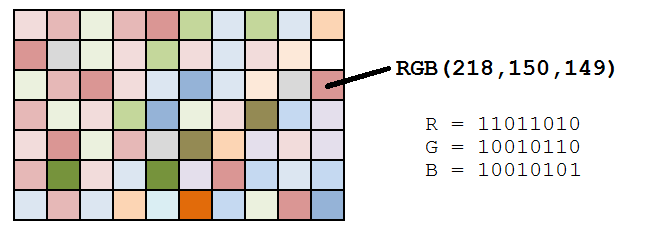
A typical computer image these days uses 24 bits to represent the color of each pixel. Eight bits are used to store the intensity of the red part of a pixel (00000000 through 11111111), giving 256 distinct values. Eight bits are used to store the green component, and eight bits are used to store the blue component.

Each pixel has a coordinate pair (x,y) describing its position on two orthogonal axes from defined origin O.It is around this origin we are going to rotate this image.What we need to do is take the RGB values at every (x,y) location, rotate it as needed, and then write these values in the new location, considering (x,y) with respect to the origin we assumed.The new location is obtained by using the transformation matrix.

When image will be rotated ,the dimension of the frame containing it will change so to find the new dimensions we use this formula,
new_width=|old_width×cosθ|+|old_height×sinθ|
new_height=|old_height×cosθ|+ |old_row×sinθ|
now let’s code it
import numpy as np
from PIL import Image
import math


image = np.array(Image.open("test.png"))             # Load the image
angle=int(input("Enter the angle :- "))                # Ask the user to enter the angle of rotation

# Define the most occuring variables
angle=math.radians(angle)                               #converting degrees to radians
cosine=math.cos(angle)
sine=math.sin(angle)
height=image.shape[0]                                   #define the height of the image
width=image.shape[1]                                    #define the width of the image

# Define the height and width of the new image that is to be formed
new_height  = round(abs(image.shape[0]*cosine)+abs(image.shape[1]*sine))+1
new_width  = round(abs(image.shape[1]*cosine)+abs(image.shape[0]*sine))+1

# define another image variable of dimensions of new_height and new _column filled with zeros
output=np.zeros((new_height,new_width,image.shape[2]))

# Find the centre of the image about which we have to rotate the image
original_centre_height   = round(((image.shape[0]+1)/2)-1)    #with respect to the original image
original_centre_width    = round(((image.shape[1]+1)/2)-1)    #with respect to the original image

# Find the centre of the new image that will be obtained
new_centre_height= round(((new_height+1)/2)-1)        #with respect to the new image
new_centre_width= round(((new_width+1)/2)-1)          #with respect to the new image

for i in range(height):
    for j in range(width):
        #co-ordinates of pixel with respect to the centre of original image
        y=image.shape[0]-1-i-original_centre_height
        x=image.shape[1]-1-j-original_centre_width

        #co-ordinate of pixel with respect to the rotated image
        new_y=round(-x*sine+y*cosine)
        new_x=round(x*cosine+y*sine)

        '''since image will be rotated the centre will change too,
           so to adust to that we will need to change new_x and new_y with respect to the new centre'''
        new_y=new_centre_height-new_y
        new_x=new_centre_width-new_x

        # adding if check to prevent any errors in the processing
        if 0 <= new_x < new_width and 0 <= new_y < new_height and new_x>=0 and new_y>=0:
            output[new_y,new_x,:]=image[i,j,:]                          #writing the pixels to the new destination in the output image

pil_img=Image.fromarray((output).astype(np.uint8))                       # converting array to image
pil_img.save("rotated_image.png")                                                 # saving the image

ALIASING
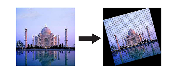
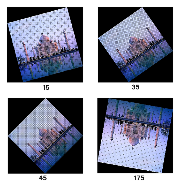
So our resultant image is rotated by 15 degrees ,so it really worked,but what are those black dots?This is a problem called aliasing.Multiplying by sines and cosines on the integer coordinates of the source image gives real number results, and these have to be rounded back to integers again to be plotted. Sometimes this number rounding means the same destination location is addressed more than once, and sometimes certain pixels are missed completely. When the pixels are missed, the background shows through. This is why there are holes.The aliasing problem gets worse when angles are closesr to the diagonals. Here are a few examples of images at different rotations:

What can we do about this? There are a variety of solutions. One of them is to oversample the source image. We can pretend that each of the original source pixels is really a grid of n x n smaller pixels (all of the same color), and calculate the destination coordinates of each of these subpixels and plot these
A more refined way is called Area Mapping. For this, you invert the problem, and for each destination pixel, you find which four partial source pixels that it was created from. The color for the destination is calculated by the area-weighted average of the four source pixels (The source pixels that contribute more to the destination pixel have a greater influence on its color). This algorithm not only ensures that there are no gaps in the destination, but also appropriately averages the colors (ensuring both a smoother image and also keeping the average brightness of the rotated image constant).
However, there is a more elegant method, and this is the method that was used many years ago when computing power (and memory) were at a premium and every processor cycle worth its weight in gold. It is called the three shear rotation method.
THREE SHEARS
These method works by expanding 2D rotation matrix into three different matrices.

There are some interesting properties of this matrix:-
- The three matrices are all shear matrices
- The first and the last matrices are the same
- The determinant of each matrix is same (each stage is conformal and keeps the area the same).
- As the shear happens in just one plane at time, and each stage is conformal in area, no aliasing gaps appear in any stage.
note: Shear matrix shown above rotates in clockwise direction so we need to take angle in negative values to assess for that.
So let’s code the shear transformation
import numpy as np
from PIL import Image
import math


def shear(angle,x,y):
    '''
    |1  -tan(????/2) |  |1        0|  |1  -tan(????/2) |
    |0      1     |  |sin(????)   1|  |0      1     |

    '''
    # shear 1
    tangent=math.tan(angle/2)
    new_x=round(x-y*tangent)
    new_y=y

    #shear 2
    new_y=round(new_x*math.sin(angle)+new_y)      #since there is no change in new_x according to the shear matrix

    #shear 3
    new_x=round(new_x-new_y*tangent)              #since there is no change in new_y according to the shear matrix

    return new_y,new_x


image = np.array(Image.open("test.png"))             # Load the image
angle=-int(input("Enter the angle :- "))                # Ask the user to enter the angle of rotation

# Define the most occuring variables
angle=math.radians(angle)                               #converting degrees to radians
cosine=math.cos(angle)
sine=math.sin(angle)

height=image.shape[0]                                   #define the height of the image
width=image.shape[1]                                    #define the width of the image

# Define the height and width of the new image that is to be formed
new_height  = round(abs(image.shape[0]*cosine)+abs(image.shape[1]*sine))+1
new_width  = round(abs(image.shape[1]*cosine)+abs(image.shape[0]*sine))+1

# define another image variable of dimensions of new_height and new _column filled with zeros
output=np.zeros((new_height,new_width,image.shape[2]))
image_copy=output.copy()


# Find the centre of the image about which we have to rotate the image
original_centre_height   = round(((image.shape[0]+1)/2)-1)    #with respect to the original image
original_centre_width    = round(((image.shape[1]+1)/2)-1)    #with respect to the original image

# Find the centre of the new image that will be obtained
new_centre_height= round(((new_height+1)/2)-1)        #with respect to the new image
new_centre_width= round(((new_width+1)/2)-1)          #with respect to the new image


for i in range(height):
    for j in range(width):
        #co-ordinates of pixel with respect to the centre of original image
        y=image.shape[0]-1-i-original_centre_height
        x=image.shape[1]-1-j-original_centre_width

        #Applying shear Transformation
        new_y,new_x=shear(angle,x,y)

        '''since image will be rotated the centre will change too,
            so to adust to that we will need to change new_x and new_y with respect to the new centre'''
        new_y=new_centre_height-new_y
        new_x=new_centre_width-new_x

        output[new_y,new_x,:]=image[i,j,:]                          #writing the pixels to the new destination in the output image


pil_img=Image.fromarray((output).astype(np.uint8))                       # converting array to image
pil_img.save("rotated_image.png")                                                 # saving the image

In the first shear operation, raster columns are simply shifted up and down relative to each other. The shearing is symmetric around the center of the image. It’s analogous to shearing a deck of playing cards.
The second shear operation does a similar thing on the previous image, but this time does the shearing left to right.
The final shear is the same as the first operation; this time applied to the intermediate image.
No gaps! How elegant is that? We just rotated an image an arbitrary amount (smoothly) using three shear operations!
In times-past, when floating point and trig calculations were expensive, these properties were very important. Because only one plane was being modified at once, no additional memory was needed as the code could simple walk down the raster line making the changes it needed. Pretty cool
This article has been published from the source link without modifications to the text. Only the headline has been changed.


