We introduce the weightwatcher (ww) , a python tool for a python tool for computing quality metrics of trained, and pretrained, Deep Neural Netwworks.
pip install weightwatcher
This blog describes how to use the tool in practice; see our most recent paper for even more details.
Here is an example with pretrained VGG11 from pytorch (ww works with keras models also):
import weightwatcher as ww
import torchvision.models as models

model = models.vgg11(pretrained=True)
watcher = ww.WeightWatcher(model=model)
results = watcher.analyze()

summary = watcher.get_summary()
details = watcher.get_details()
WeightWatcher generates a dict that summarizes the empirical quality metrics for the model (with the most useful metrics)
summary: = { ...
  alpha: 2.572493
  alpha_weighted: 3.418571
  lognorm: 1.252417
  logspectralnorm: 1.377540
  logpnorm: 3.878202
... }
The tool also generates a details pandas dataframe, with a layer-by-layer analysis (shown below)
The summary contains the Power Law exponent (), as well as several log norm metrics, as explained in our papers, and below. Each value represents an empirical quality metric that can be used to gauge the gross effectiveness of the model, as compared to similar models.
(The main weightwatcher notebook demonstrates more features )
For example, lognorm is the average over all layers L of the log of the Frobenius norm of each layer weight matrix :
lognorm: average log Frobenius Norm :=
Where the individual layer Frobenius norm, for say a Fully Connected (FC layer, may be computed as
np.log10(np.linalg.norm(W))
Comparing Metrics Across Models:
We can use these metrics to compare models across a common architecture series, such as the VGG series, the ResNet series, etc. These can be applied to trained models, pretrained models, and/or even fine-tuned models.
Consider the series of models VGG11, VGG11_BN, … VGG19, VGG_19, available in pytorch. We can plot the reported the various log norm metrics vs the reported test accuracies.
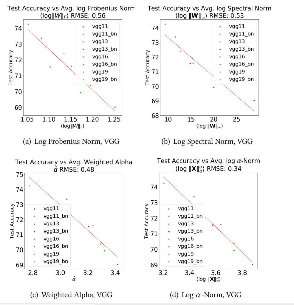
For a series of similar, well-trained models, all of the empirical log norm metrics correlate well with the reported test accuracies! Moreover, the Weighted Alpha and Log Norm metrics work best.
Smaller is better.
We also run a ordinary linear regression (OLS) and the root mean squared error (RMSE) , and for several other CV models that are available in the pytorch torchvision.models package.
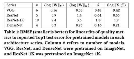
We have tested this on over 100 well trained computer vision (CV) pre-trained models on multiple data sets (such as the ImageNet-1K subset of ImageNet). These trends how for nearly every case of well-trained models.
Notice that the RMSE for ResNet, trained on ImageNet1K, is larger than for ResNet trained on the full ImageNet, even though ResNet-1K has more models in the regression. that (19 vs 5). For the exact same model, the larger and better data set shows a better OLS fit!
How can you use this ?
We have several ideas where we hope this would be useful. These include:
- comparing different models trained using Auto-ML (in addition to standard cross-validation)
- judging the quality of NLP models for generating fake text (in addition to, say, the perplexity)
- evaluating different unsupervised clustering models, to determine which (presumably) gives the best clusters
- deciding if you have enough data, or need to add more, for your specific model or series of models.
Detailed quality metrics: layer-by-layer
We can learn even more about a model by looking at the empirical metrics, layer by layer. The results is a dataframe that contains empirical quality metrics for each layer of the model. An example output, for VGG11, is:
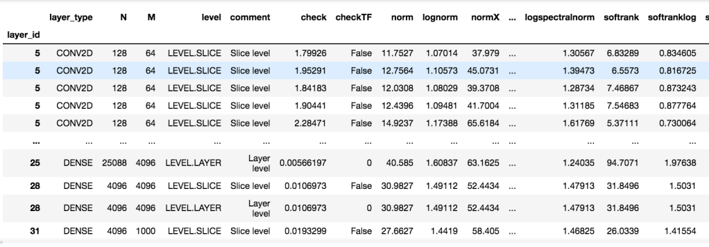
The columns contain both metadata for each layer (id, type, shape, etc), and the values of the empirical quality metrics for that layer matrix.
These metrics depend on the spectral properties–singular values of
, or, equivalently, the eigenvalues
of the correlation matrix of
.
The Power Law Exponent 
WeightWatcher is unique in that it can measure the amount of correlation, or information, that a model contains–without peeking at the training or test data. Data Correlation is measured by the Power Law (PL) exponents .
WeightWatcher computes the eigenvalues (by SVD) for each layer weight matrix , and fits the eigenvalue density (i.e. histogram
to a truncated Power Law (PL), with PL exponent
In nearly every pretrained model we have examined, the Empirical Spectral Density can be fit to a truncated PL. And the PL exponent usually is in the range , where smaller is better.
Here is an example of the output of weightwatcher of the second Fully Connected layer (FC2) in VGG11. These results can be reproduced using the WeightWatcher-VGG.ipynb notebook in the ww-trends-2020 github repo., using the options:
|
1
|
results = watcher.analyze(alphas=True, plot=True) |
The plot below shows the ESD (Empirical Spectral Density ,), of the weight matrix
, in layer FC2. Again, this is a (normalized) histogram of the eigenvalues
of the correlation matrix
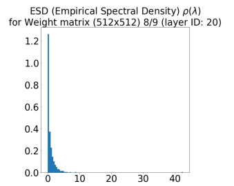
The FC2 matrix is square, 512×512, and has an aspect ratio of Q=N/M=1 . The maximum eigenvalue is about 45, which is typical for many heavy tailed ESDs. And there is a large peak at 0, which is normal for Q=1. Because Q= 1, the ESD might look heavy tailed, but this can be deceiving because a random matrix with Q=1 would look similar. Still, as with nearly all well-trained DNNS, we expect the FC2 ESD to be well fit by a Power Law model, with an exponent
(i.e. in the Fat Tailed Universality class), or at least, for a model that is not ‘flawed’ in some way,
.
alpha . PL exponent for for W:
The smaller alpha is , for each layer, the more correlation that layer describes. Indeed, in the best performing models, all of the layer alphas approach 2
.
To check that the ESD is really heavy tailed, we need to check the Power Law (PL) fit. This is done by inspecting the weightwatcher plots.
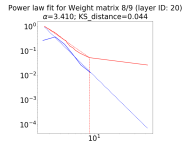
The plot on the right shows the output of the powerlaw package, which is used to do the PL fit of the ESD. The PL exponent , which is a typical value for (moderately, i.e. Fat) Heavy Tailed ESDs. Also, the KS distance is small
, which is good. We can also see this visually. The dots are the actual data, and the lines are the fits. If the lines are reasonably straight, and match the dots, and in the range
the fit is good. And they are. This is a good PL fit.
Good Model, Bad Data ?
As shown above, with ResNet vs ResNet-1K, the weightwatcher tool can help you decide if you have enough data, or your model/architecture would benefit from more data. Indeed, poorly trained models, with very bad data sets, show strange behavior that you can detect using weightwatcher
Here is an example of the infamous OpenAI GPT model, originally released as a poorly-trained model –so it would not be misused. It was too dangerous to release ? We can compare this deficient GPT with the new and improved GPT2-small model, which has basically the same architecture, but has been trained as well as possible. Yes, they gave in an released it! (Both are in the popular huggingface package, and weightwatcher can read and analyze these models) Below, we plot a histogram of the PL exponents , as well as histogram of the log Spectral Norms
for each layer in GPT (blue) and GPT2 (red)
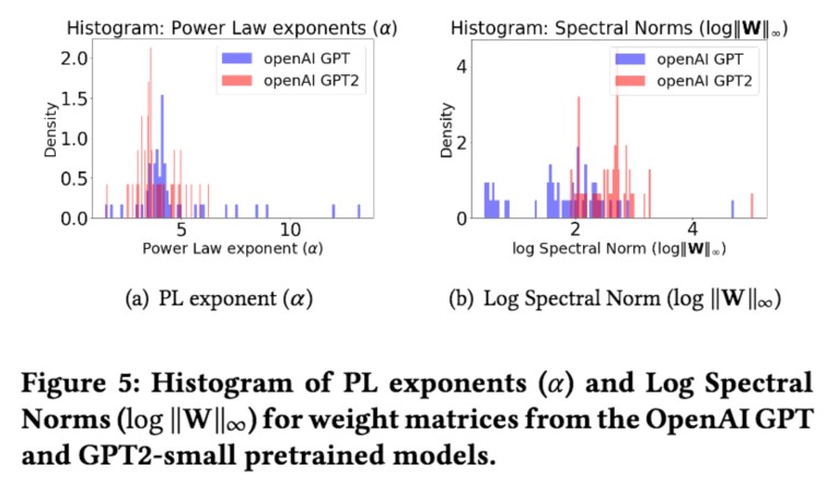
These results can be reproduced using the WeightWatcher-OpenAI-GPT.ipynb notebook in the ww-trends-2020 github repo.
Notice that the poorly-trained GPT model has many unusually high values of alpha . Many are be above 6, and even range upto 10 or 12 ! This is typical of poorly trained and/or overparameterized models.
Notice that the new and improved GPT2-small does not have the unusually high PL exponents any more, and, also, the peak of the histogram distribtion is farther to the left (smaller).
Smaller alpha is always better.
If you have a poorly trained model. and you fix your model by adding more and better data, the alphas will generally settle down to below 6. Note: this can not be seen in a total average because the large values will throw the average off–to see this, make a histogram plot of alpha
What about the log Spectral Norm ? It seems to show inconsistent behavior. Above, we saw that smaller
is better. But now it looks as if smaller
is worse ? What is going on with this…and the other empirical Norm metrics ?
Now let’s take a deeper look at how to use the empirical log Norm metrics:
Norm Metrics: 
Unlike the PL exponent alpha, the empirical Norm metrics depend strongly on the scale of the weight matrix W. As such, they are highly sensitive to problems like Scale Collapse–and examining these metrics can tell us when something is potentially very wrong with our models.
First, what are we looking at ? These empirical (log) Norm metrics reported are defined using the raw eigenvalues. We can compute the eigenvalues of X pretty easily (although actually in the code we compute the singular values of W using the sklearn TruncatedSVD method.)
|
1
2
3
4
5
|
M = np.min(W.shape)svd = TruncatedSVD(n_components=M-1)svd.fit(W)sv = svd.singular_values_eigen_values = sv*sv |
Recall that the Frobenius norm (squared) for matrix W is also the sum of the eigenvalues of X. The Spectral Norm (squared) is just the maximum eigenvalue of X. The weighted alpha
and the log
(or Shatten) Norm are computed after fitting the PL exponent
for the layer. In math, these are:
- lognorm:
- logspectralnorm:
- alpha_weighted:
- logpnorm:
The weightwatcher code computes the necessary eigenvalues, does the PowerLaw (PL) fits, and reports these, and other, empirical quality metrics, for you, both for the average (summary) and layer-by-layer (details) of each. The details dataframe has many more metrics as well, but, for now we will focus on these four.
Now, what can we do with them? We are going to look at 3 ways to identify potential problems in a DNN, which can not be seen by just looking at the test accuracy
- Correlation Flow : comparing different architectures
- Alpha Spikes : Identifying overparameterized models
- Scale Collapse : potential problems when distilling models
Correlation Flow : comparing different architectures
Using the weighwatcher details dataframe, we can plot the PL exponent alpha vs. the layer Id to get what is called a Correlation Flow plot:
Let us do this, by comparing 3 common (pretrained) computer vision models: VGG, ResNet, and DenseNet.
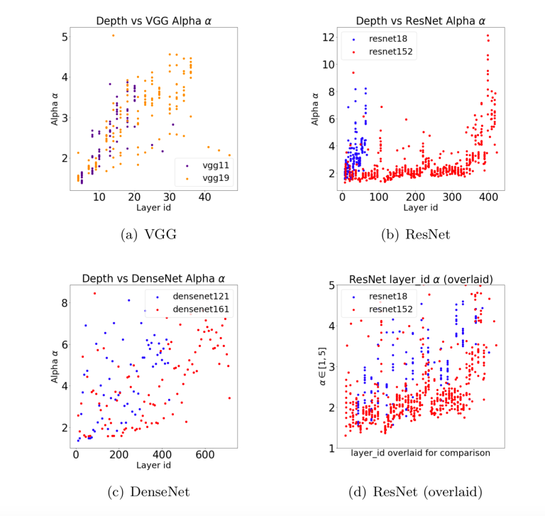
These results can be reproduced using the following notebooks:
Recall that good models have average PL exponents , in the Fat Tailed Universality class. Likewise, we find that, if we plot alpha vs layer_id, then good models also have stable alphas, in this range.
The VGG11 and 19 models have good alphas, all within the Fat Tailed Universality class, or smaller. And both the smaller and larger models show similar behavior. Also, noitce that the last 3 and FC layers in the VGG models all have final smaller alphas, . So while the alphas are increasing as we move down the model, the final FC layers seem to capture and concentrate the information, leading to more correlated layer weight matrices at the end.
ResNet152 is an even better example of good Correlation Flow. It has a large number of alphas near 2, contiguously, for over 200 layers. Indeed, ResNet models have been trained with over 1000 layers; clearly the ResNet architecture supports a good flow of information.
Good Correlation Flow shows that the DNN architecture is learning the correlations in the data at every layer, and implies (*informally) that information is flowing smoothly through the network.
Good DNNs show good Correlation Flow
We also find that models in an architecture series (VGG, ResNet, DenseNet, etc) all have similar Correlation Flow patterns, when adjusting for the model depth.
Bad models, however, have alphas that increase with layer_id, or behave erratically. This means that the information is not flowing well through the network, and the final layers are not fully correlated. For example, the older VGG models have alphas in a good range, but, as we go down the network, the alphas are systematically increasing. The final FC layers fix the problem, although, maybe a few residual connections, like in ResNet, might improve these old models even more.
You might think adding a lot of residual connections would improve Correlation Flow–but too many connections is also bad. The DenseNet series is an example of an architecture with too many residual connections. Here, both with the pretrained DenseNet126 and 161 we see the many , and, looking down the network layers, the are scattered all over. The Correlation Flow is poor and even chaotic, and, we conjecture, less than optimal.
Curiously, the ResNet models show good flow internally, as shown when we zoom-in, in (d) above. But the last few layers have unusually large alphas; we will discuss this phenomena now.
Advice: If you are training or finetuning a DNN model for production use, use weightwatcher to plot the Correlation Flow. If you see alphas increasing with depth, behaving chaotically, or there are just a lot of alphas >> 6, revisit your architecture and training procedures.
Alpha Spikes : Identifying overparameterized models
When is a DNN is over-parameterized, once trained on some data ?
Easy…just look at alphas. We have found that well-trained, or perhaps fully-trained, models, should have . And the best CV models have most of their alphas just above 2.0. However, some models, such as NLP OpenAI GPT2 and BERT models, have a wider
. And many models have several unusually large alphas, with latex \alpha\gg 6$. What is going on ? And how is it useful ?
The current batch of NLP Transformer models are great examples. We suspect that many models, like BERT and GPT-xl, are over-parameterized, and that to fully use them in production, they need to be fine-tuned. Indeed, that is the whole point of these models; NLP transfer learning.
Let’s take a look the current crop of pretrained OpenAI GPT-2 models, provided by the huggingface package. We call these “good-better-best” series.
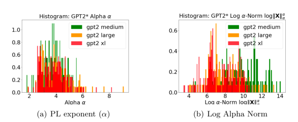
These results can be reproduced using the WeightWatcher-OpenAI-GPT2.ipynb notebook.
For both the PL exponent (a) and our Log Alpha Norm (b) , Smaller is Better. The latest and greatest OpenAI GPT2-xl model (in red) has both smaller alphas and smaller empirical log norm metrics, compared to the earlier GP2-large (orange) and GPT2-medium (green) models.
But the GPT2-xl model also has more outlier alphas:
We have seen similar behavior in other NLP models, such as comparing OpenAI GPT to GPT2-small, and the original BERT, as compared to the Distilled Bert (as discussed in my recent Stanford Lecture). We suspect that when these large NLP Trasnformer models are fine-tuned or distilled, the alphas will get smaller, and performance will improve.
Advice: So when you fine-tune your models, monitor the alphas with weightwatcher. If they do not decrease enough, add more data, and/or try to improve the training protocols.
But you also have to be careful not to break your model, as have found that some distillation methods may do this.
Scale Collapse : When Models Go Bad
Frequently one may finetune a model, for transfer learning, distillation, or just to add more data.
How can we know if we broke the model ?
We have found that poorly trained models frequently exhibit Scale Collapse, in which 1 or more layers have unusually small Spectral and/or Frobenius Norms.
This can be seen in your models by running plotting a histogram of the logspectralnorm column from the details dataframe
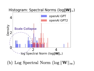
Recall earlier we noted the poorly-trained in the OpenAI GPT model. This is typical of many porly-trained models. Because of this, log norm metrics can not be reliable used to predict trends in accuracies on poorly-trained models.
However, we can use the empirical log Norm metrics to detect problems that can not be seen by simply looking at the training and test accuracies.
Distillation may break models: be careful out there
We have also observed this in some distilled models. Below we look at the ResNet20 model, before and after distillation using the Group Regularization method (as described in the Intel distiller package and provided in the model zoo). We plot the Spectral Norm (maximum eigenvalue) and PL exponent alpha vs. the layer_id (depth) for both the baseline (green) and finetuned /distiller (red) ResNet20 models.
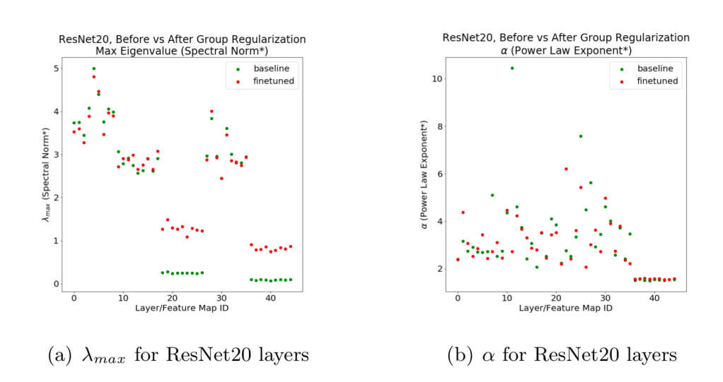

These results can be reproduced by installing the distiller package, downloading the model zoo pretrained models, and running the WeightWatcher-Intel-Distiller-ResNet20.ipynb notebook in the distiller folder. (We do note that these are older results, and we used older versions of both distiller and weighwatcher, which used a different normalization on the Conv2D layers. Current results may differ although we expect to see similar trends.)
Notice that the baseline and finetuned ResNet20 have similar PL exponents (b) for all layers, but for several layers in (a), the Spectral Norm (maximum eigenvalue) collapses in value. That is, the Scale Collapses. This is bad, and characteristic of a poorly trained model like the original GPT.
Advice: if you finetune a model, use weighwatcher to monitor the log Spectral Norms. If you see unusually small values, something is wrong.
Learn More about the WeightWatcher tool
Our latest paper is now on archive.
Please check out the github webpage for WeightWatcher and the associated papers and online talks at Stanford, UC Berkeley, and the wonderful podcasts that have invited us on to speak about the work.
This article has been published from the source link without modifications to the text. Only the headline has been changed.


