In this post, I’m going to implement standard logistic regression from scratch in Python. Logistic regression is a generalized linear model that we can use to model or predict categorical outcome variables. For example, we might use logistic regression to predict whether someone will be denied or approved for a loan, but probably not to predict the value of someone’s house.

So, how does it work? In logistic regression, we’re essentially trying to find the weights that maximize the likelihood of producing our given data and use them to categorize the response variable. Maximum Likelihood Estimation is a well covered topic in statistics courses and it is extremely useful.

Since the likelihood maximization in logistic regression doesn’t have a closed form solution, I’ll solve the optimization problem with gradient ascent. Gradient ascent is the same as gradient descent, except I’m maximizing instead of minimizing a function. Before I do any of that, though, I need some data.

Generating Data

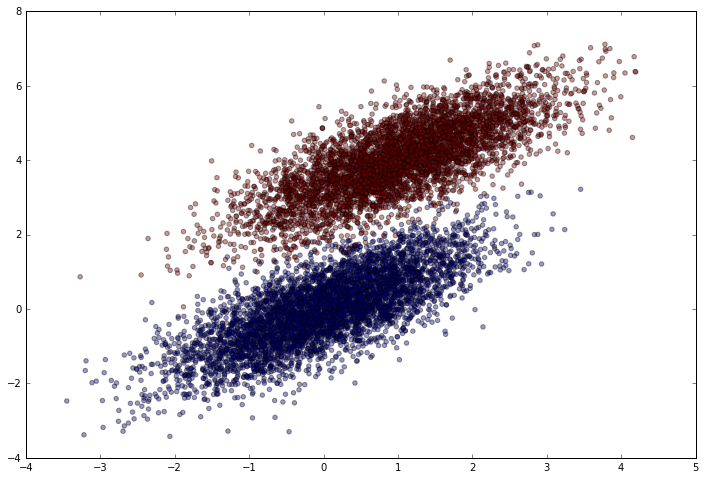
Like I did in my post on building neural networks from scratch, I’m going to use simulated data. I can easily simulate separable data by sampling from a multivariate normal distribution.

import numpy as np
import matplotlib.pyplot as plt
%matplotlib inline

np.random.seed(12)
num_observations = 5000

x1 = np.random.multivariate_normal([0, 0], [[1, .75],[.75, 1]], num_observations)
x2 = np.random.multivariate_normal([1, 4], [[1, .75],[.75, 1]], num_observations)

simulated_separableish_features = np.vstack((x1, x2)).astype(np.float32)
simulated_labels = np.hstack((np.zeros(num_observations),
                              np.ones(num_observations)))

Let’s see how it looks.

plt.figure(figsize=(12,8))
plt.scatter(simulated_separableish_features[:, 0], simulated_separableish_features[:, 1],
            c = simulated_labels, alpha = .4)

Picking a Link Function

Generalized linear models usually tranform a linear model of the predictors by using a link function. In logistic regression, the link function is the sigmoid. We can implement this really easily.

def sigmoid(scores):
    return 1 / (1 + np.exp(-scores))

Maximizing the Likelihood

To maximize the likelihood, I need equations for the likelihood and the gradient of the likelihood. Fortunately, the likelihood (for binary classification) can be reduced to a fairly intuitive form by switching to the log-likelihood. We’re able to do this without affecting the weights parameter estimation because log transformations are monotonic.

For anyone interested in the derivations of the functions I’m using, check out Section 4.4.1 of Hastie, Tibsharani, and Friedman’s Elements of Statistical Learning. For those less comfortable reading math, Carlos Guestrin (Univesity of Washington) has a fantastic walkthrough of one possible formulation of the likelihood and gradient in a series of short lectures on Coursera.

Calculating the Log-Likelihood

The log-likelihood can be viewed as a sum over all the training data. Mathematically,

$$ll=\sum _{i=1}^N{y}_i{\beta }^T{x}_i-log(1+e^{{\beta }^{}{x}_i})$$

where $y$ is the target class (0 or 1), $x_i$ is an individual data point, and $\beta$ is the weights vector.

I can easily turn that into a function and take advantage of matrix algebra.

def log_likelihood(features, target, weights):
    scores = np.dot(features, weights)
    ll = np.sum( target*scores - np.log(1 + np.exp(scores)) )
    return ll

Calculating the Gradient

Now I need an equation for the gradient of the log-likelihood. By taking the derivative of the equation above and reformulating in matrix form, the gradient becomes:

$$▽ll=X^T(Y-Predictions)$$

Like the other equation, this is really easy to implement. It’s so simple I don’t even need to wrap it into a function.

Building the Logistic Regression Function

Finally, I’m ready to build the model function. I’ll add in the option to calculate the model with an intercept, since it’s a good option to have.

def logistic_regression(features, target, num_steps, learning_rate, add_intercept = False):
    if add_intercept:
        intercept = np.ones((features.shape[0], 1))
        features = np.hstack((intercept, features))
        
    weights = np.zeros(features.shape[1])
    
    for step in xrange(num_steps):
        scores = np.dot(features, weights)
        predictions = sigmoid(scores)

        # Update weights with gradient
        output_error_signal = target - predictions
        gradient = np.dot(features.T, output_error_signal)
        weights += learning_rate * gradient
        
        # Print log-likelihood every so often
        if step % 10000 == 0:
            print log_likelihood(features, target, weights)
        
    return weights

Time to run the model.

weights = logistic_regression(simulated_separableish_features, simulated_labels,
                     num_steps = 300000, learning_rate = 5e-5, add_intercept=True)

-4346.26477915
[...]
-140.725421362
-140.725421357
-140.725421355

Comparing with Sk-Learn’s LogisticRegression

How do I know if my algorithm spit out the right weights? Well, on the one hand, the math looks right – so I should be confident it’s correct. On the other hand, it would be nice to have a ground truth.

Fortunately, I can compare my function’s weights to the weights from sk-learn’s logistic regression function, which is known to be a correct implementation. They should be the same if I did everything correctly. Since sk-learn’s LogisticRegression automatically does L2 regularization (which I didn’t do), I set C=1e15 to essentially turn off regularization.

from sklearn.linear_model import LogisticRegression

clf = LogisticRegression(fit_intercept=True, C = 1e15)
clf.fit(simulated_separableish_features, simulated_labels)

print clf.intercept_, clf.coef_
print weights

[-13.99400797] [[-5.02712572  8.23286799]]
[-14.09225541  -5.05899648   8.28955762]

As expected, my weights nearly perfectly match the sk-learn LogisticRegression weights. If I trained the algorithm longer and with a small enough learning rate, they would eventually match exactly. Why? Because gradient ascent on a concave function will always reach the global optimum, given enough time and sufficiently small learning rate.

What’s the Accuracy?

To get the accuracy, I just need to use the final weights to get the logits for the dataset (final_scores). Then I can use sigmoid to get the final predictions and round them to the nearest integer (0 or 1) to get the predicted class.

data_with_intercept = np.hstack((np.ones((simulated_separableish_features.shape[0], 1)),
                                 simulated_separableish_features))
final_scores = np.dot(data_with_intercept, weights)
preds = np.round(sigmoid(final_scores))

print 'Accuracy from scratch: {0}'.format((preds == simulated_labels).sum().astype(float) / len(preds))
print 'Accuracy from sk-learn: {0}'.format(clf.score(simulated_separableish_features, simulated_labels))

Accuracy from scratch: 0.9948
Accuracy from sk-learn: 0.9948

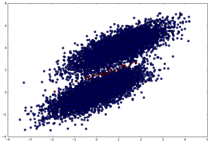
Nearly perfect (which makes sense given the data). We should only have made mistakes right in the middle between the clusters. Let’s make sure that’s what happened. In the following plot, blue points are correct predictions and red points are incorrect predictions.

plt.figure(figsize = (12, 8))
plt.scatter(simulated_separableish_features[:, 0], simulated_separableish_features[:, 1],
            c = preds == simulated_labels - 1, alpha = .8, s = 50)

Conclusion

In this post, I built a logistic regression function from scratch and compared it with sk-learn’s logistic regression function. While both functions give essentially the same result, my own function is significantly slower because sklearn uses a highly optimized solver. While I’d probably never use my own algorithm in production, building algorithms from scratch makes it easier to think about how you could design extensions to fit more complex problems or problems in new domains.

This article has been published from the source link without modifications to the text. Only the headline has been changed.

Source link