We are missing one important variable that affects Calorie_Burnage, which is the Duration of the training session.
Duration in combination with Average_Pulse will together explain Calorie_Burnage more precisely.
Linear Regression
The term regression is used when you try to find the relationship between variables.
In Machine Learning and in statistical modeling, that relationship is used to predict the outcome of events.
In this module, we will cover the following questions:
- Can we conclude that Average_Pulse and Duration are related to Calorie_Burnage?
- Can we use Average_Pulse and Duration to predict Calorie_Burnage?
Least Square Method
Linear regression uses the least square method.
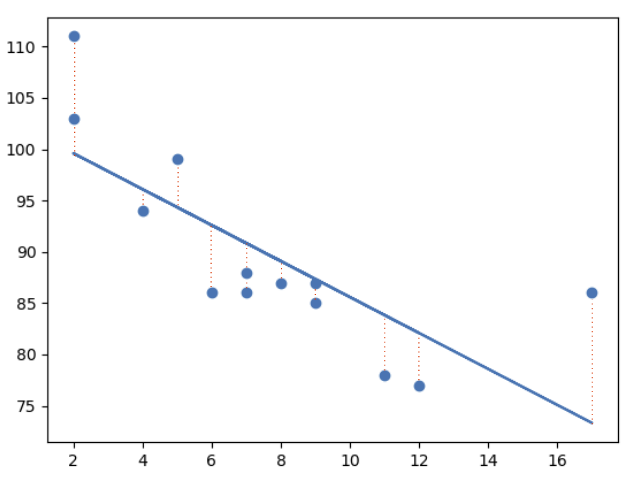
The concept is to draw a line through all the plotted data points. The line is positioned in a way that it minimizes the distance to all of the data points.
The distance is called “residuals” or “errors”.
The red dashed lines represents the distance from the data points to the drawn mathematical function.
Linear Regression Using One Explanatory Variable
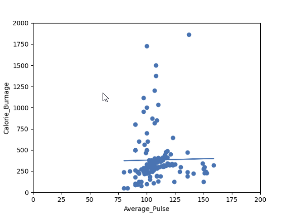
In this example, we will try to predict Calorie_Burnage with Average_Pulse using Linear Regression:
Example
import pandas as pd
import matplotlib.pyplot as plt
from scipy import stats

full_health_data = pd.read_csv("data.csv", header=0, sep=",")

x = full_health_data["Average_Pulse"]
y = full_health_data ["Calorie_Burnage"]

slope, intercept, r, p, std_err = stats.linregress(x, y)

def myfunc(x):
return slope * x + intercept

mymodel = list(map(myfunc, x))

plt.scatter(x, y)
plt.plot(x, slope * x + intercept)
plt.ylim(ymin=0, ymax=2000)
plt.xlim(xmin=0, xmax=200)
plt.xlabel("Average_Pulse")
plt.ylabel ("Calorie_Burnage")
plt.show()
Example Explained:
- Import the modules you need: Pandas, matplotlib and Scipy
- Isolate Average_Pulse as x. Isolate Calorie_burnage as y
- Get important key values with: slope, intercept, r, p, std_err = stats.linregress(x, y)
- Create a function that uses the slope and intercept values to return a new value. This new value represents where on the y-axis the corresponding x value will be placed
- Run each value of the x array through the function. This will result in a new array with new values for the y-axis: mymodel = list(map(myfunc, x))
- Draw the original scatter plot: plt.scatter(x, y)
- Draw the line of linear regression: plt.plot(x, mymodel)
- Define maximum and minimum values of the axis
- Label the axis: “Average_Pulse” and “Calorie_Burnage”
Output:
Data Science – Regression Table
Regression Table
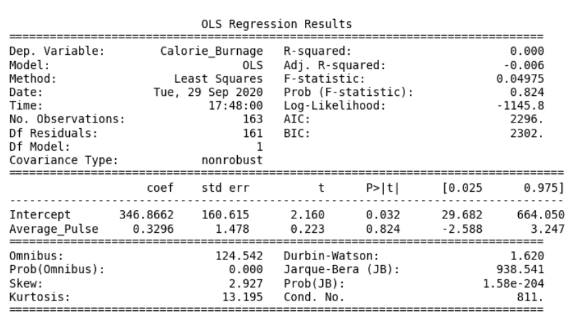
The output from linear regression can be summarized in a regression table.
The content of the table includes:
- Information about the model
- Coefficients of the linear regression function
- Regression statistics
- Statistics of the coefficients from the linear regression function
- Other information that we will not cover in this module
Regression Table with Average_Pulse as Explanatory Variable
You can now begin your journey on analyzing advanced output!
Create a Linear Regression Table in Python
Here is how to create a linear regression table in Python:
Example
import pandas as pd
import statsmodels.formula.api as smf

full_health_data = pd.read_csv("data.csv", header=0, sep=",")

model = smf.ols('Calorie_Burnage ~ Average_Pulse', data = full_health_data)
results = model.fit()
print(results.summary())
Example Explained:
- Import the library statsmodels.formula.api as smf. Statsmodels is a statistical library in Python.
- Use the full_health_data set.
- Create a model based on Ordinary Least Squares with smf.ols(). Notice that the explanatory variable must be written first in the parenthesis. Use the full_health_data data set.
- By calling .fit(), you obtain the variable results. This holds a lot of information about the regression model.
- Call summary() to get the table with the results of linear regression
Data Science – Regression Table – Info
The “Information Part” in Regression Table
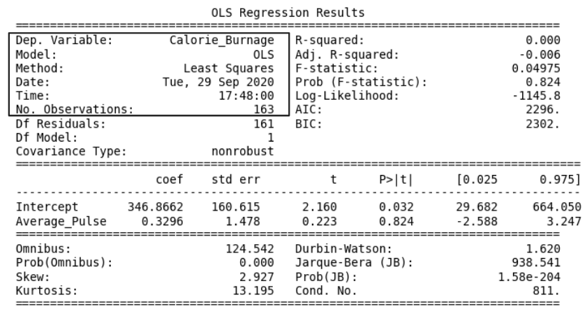
- Dep. Variable: is short for “Dependent Variable”. Calorie_Burnage is here the dependent variable. The Dependent variable is here assumed to be explained by Average_Pulse.
- Model: OLS is short for Ordinary Least Squares. This is a type of model that uses the Least Square method.
- Date: and Time: shows the date and time the output was calculated in Python.
Data Science – Regression Table – Coefficients
The “Coefficients Part” in Regression Table
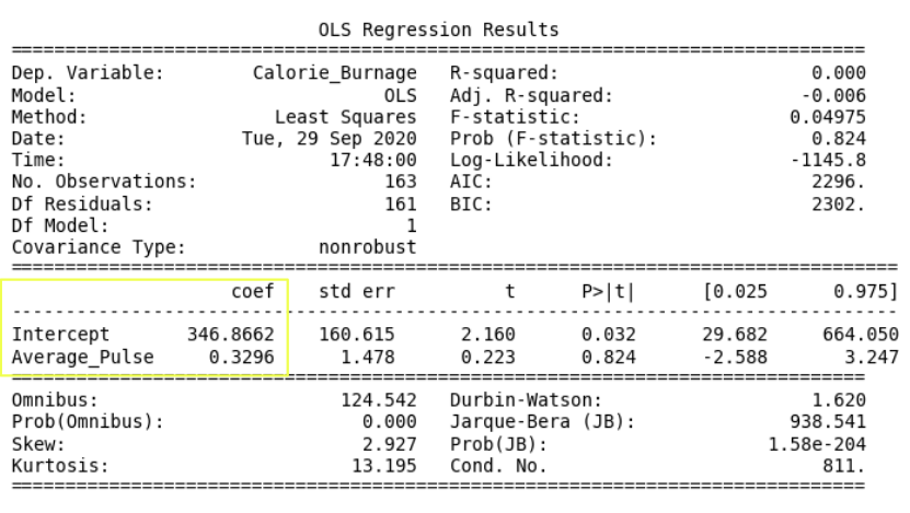
- Coef is short for coefficient. It is the output of the linear regression function.
The linear regression function can be rewritten mathematically as:
Calorie_Burnage = 0.3296 * Average_Pulse + 346.8662
These numbers means:
- If Average_Pulse increases by 1, Calorie_Burnage increases by 0.3296 (or 0,3 rounded)
- If Average_Pulse = 0, the Calorie_Burnage is equal to 346.8662 (or 346.9 rounded).
- Remember that the intercept is used to adjust the model’s precision of predicting!
Do you think that this is a good model?
Define the Linear Regression Function in Python
Define the linear regression function in Python to perform predictions.
What is Calorie_Burnage if Average_Pulse is: 120, 130, 150, 180?
Example
def Predict_Calorie_Burnage(Average_Pulse):
return(0.3296*Average_Pulse + 346.8662)

print(Predict_Calorie_Burnage(120))
print(Predict_Calorie_Burnage(130))
print(Predict_Calorie_Burnage(150))
print(Predict_Calorie_Burnage(180))
Data Science – Regression Table: P-Value
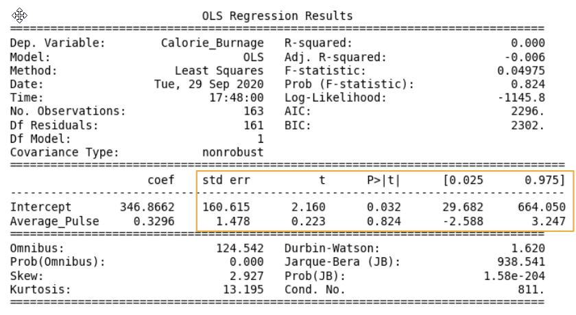
Now, we want to test if the coefficients from the linear regression function has a significant impact on the dependent variable (Calorie_Burnage).
This means that we want to prove that it exists a relationship between Average_Pulse and Calorie_Burnage, using statistical tests.
There are four components that explains the statistics of the coefficients:
- std err stands for Standard Error
- t is the “t-value” of the coefficients
- P>|t| is called the “P-value”
- [0.025 0.975] represents the confidence interval of the coefficients
We will focus on understanding the “P-value” in this module.
The P-value
The P-value is a statistical number to conclude if there is a relationship between Average_Pulse and Calorie_Burnage.
We test if the true value of the coefficient is equal to zero (no relationship). The statistical test for this is called Hypothesis testing.
- A low P-value (< 0.05) means that the coefficient is likely not to equal zero.
- A high P-value (> 0.05) means that we cannot conclude that the explanatory variable affects the dependent variable (here: if Average_Pulse affects Calorie_Burnage).
- A high P-value is also called an insignificant P-value.
Hypothesis Testing
Hypothesis testing is a statistical procedure to test if your results are valid.
In our example, we are testing if the true coefficient of Average_Pulse and the intercept is equal to zero.
Hypothesis test has two statements. The null hypothesis and the alternative hypothesis.
- The null hypothesis can be shortly written as H0
- The alternative hypothesis can be shortly written as HA
Mathematically written:
H0: Average_Pulse = 0
HA: Average_Pulse ≠ 0
H0: Intercept = 0
HA: Intercept ≠ 0
The sign ≠ means “not equal to”
Hypothesis Testing and P-value
The null hypothesis can either be rejected or not.
If we reject the null hypothesis, we conclude that it exist a relationship between Average_Pulse and Calorie_Burnage. The P-value is used for this conclusion.
A common threshold of the P-value is 0.05.
Note: A P-value of 0.05 means that 5% of the times, we will falsely reject the null hypothesis. It means that we accept that 5% of the times, we might falsely have concluded a relationship.
If the P-value is lower than 0.05, we can reject the null hypothesis and conclude that it exist a relationship between the variables.
However, the P-value of Average_Pulse is 0.824. So, we cannot conclude a relationship between Average_Pulse and Calorie_Burnage.
It means that there is a 82.4% chance that the true coefficient of Average_Pulse is zero.
The intercept is used to adjust the regression function’s ability to predict more precisely. It is therefore uncommon to interpret the P-value of the intercept.
Data Science – Regression Table: R-Squared
R – Squared
R-Squared and Adjusted R-Squared describes how well the linear regression model fits the data points:
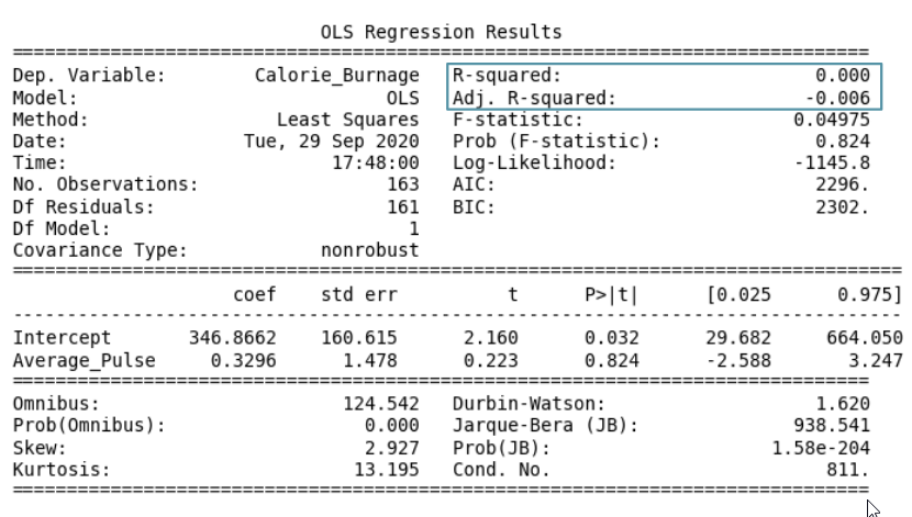
The value of R-Squared is always between 0 to 1 (0% to 100%).
- A high R-Squared value means that many data points are close to the linear regression function line.
- A low R-Squared value means that the linear regression function line does not fit the data well.
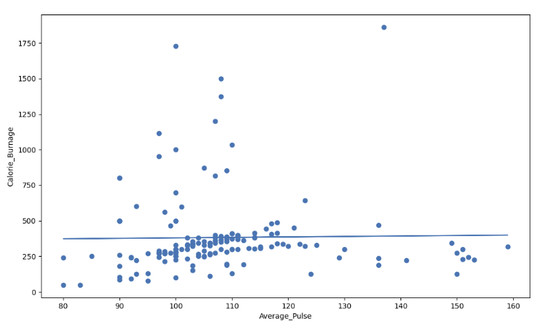
Visual Example of a Low R – Squared Value (0.00)
Our regression model shows a R-Squared value of zero, which means that the linear regression function line does not fit the data well.
This can be visualized when we plot the linear regression function through the data points of Average_Pulse and Calorie_Burnage.
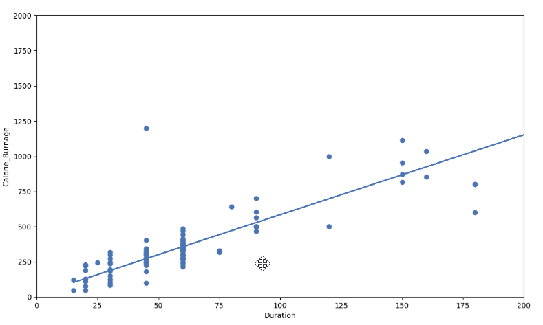
Visual Example of a High R – Squared Value (0.79)
However, if we plot Duration and Calorie_Burnage, the R-Squared increases. Here, we see that the data points are close to the linear regression function line:
Here is the code in Python:
Example
import pandas as pd
import matplotlib.pyplot as plt
from scipy import stats

full_health_data = pd.read_csv("data.csv", header=0, sep=",")

x = full_health_data["Duration"]
y = full_health_data ["Calorie_Burnage"]

slope, intercept, r, p, std_err = stats.linregress(x, y)

def myfunc(x):
return slope * x + intercept

mymodel = list(map(myfunc, x))

print(mymodel)

plt.scatter(x, y)
plt.plot(x, mymodel)
plt.ylim(ymin=0, ymax=2000)
plt.xlim(xmin=0, xmax=200)
plt.xlabel("Duration")
plt.ylabel ("Calorie_Burnage")

plt.show()
Summary – Predicting Calorie_Burnage with Average_Pulse
How can we summarize the linear regression function with Average_Pulse as explanatory variable?
- Coefficient of 0.3296, which means that Average_Pulse has a very small effect on Calorie_Burnage.
- High P-value (0.824), which means that we cannot conclude a relationship between Average_Pulse and Calorie_Burnage.
- R-Squared value of 0, which means that the linear regression function line does not fit the data well.
Data Science – Linear Regression Case
Case: Use Duration + Average_Pulse to Predict Calorie_Burnage
Create a Linear Regression Table with Average_Pulse and Duration as Explanatory Variables:
Example
import pandas as pd
import statsmodels.formula.api as smf

full_health_data = pd.read_csv("data.csv", header=0, sep=",")

model = smf.ols('Calorie_Burnage ~ Average_Pulse + Duration', data = full_health_data)
results = model.fit()
print(results.summary())
Example Explained:
- Import the library statsmodels.formula.api as smf. Statsmodels is a statistical library in Python.
- Use the full_health_data set.
- Create a model based on Ordinary Least Squares with smf.ols(). Notice that the explanatory variable must be written first in the parenthesis. Use the full_health_data data set.
- By calling .fit(), you obtain the variable results. This holds a lot of information about the regression model.
- Call summary() to get the table with the results of linear regression.
Output:
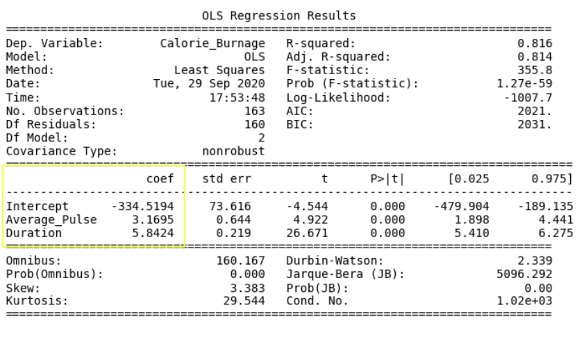
The linear regression function can be rewritten mathematically as:
Calorie_Burnage = Average_Pulse * 3.1695 + Duration * 5.8424 – 334.5194
Rounded to two decimals:
Calorie_Burnage = Average_Pulse * 3.17 + Duration * 5.84 – 334.52
Define the Linear Regression Function in Python
Define the linear regression function in Python to perform predictions.
What is Calorie_Burnage if:
- Average pulse is 110 and duration of the training session is 60 minutes?
- Average pulse is 140 and duration of the training session is 45 minutes?
- Average pulse is 175 and duration of the training session is 20 minutes?
Example
def Predict_Calorie_Burnage(Average_Pulse, Duration):
 return(3.1695*Average_Pulse + 5.8434 * Duration - 334.5194)

print(Predict_Calorie_Burnage(110,60))
print(Predict_Calorie_Burnage(140,45))
print(Predict_Calorie_Burnage(175,20))
The Answers:
- Average pulse is 110 and duration of the training session is 60 minutes = 365 Calories
- Average pulse is 140 and duration of the training session is 45 minutes = 372 Calories
- Average pulse is 175 and duration of the training session is 20 minutes = 337 Calories
Access the Coefficients
Look at the coefficients:
- Calorie_Burnage increases with 3.17 if Average_Pulse increases by one.
- Calorie_Burnage increases with 5.84 if Duration increases by one.
Access the P-Value
Look at the P-value for each coefficient.
- P-value is 0.00 for Average_Pulse, Duration and the Intercept.
- The P-value is statistically significant for all of the variables, as it is less than 0.05.
So here we can conclude that Average_Pulse and Duration has a relationship with Calorie_Burnage.
Adjusted R-Squared
There is a problem with R-squared if we have more than one explanatory variable.
R-squared will almost always increase if we add more variables, and will never decrease.
This is because we are adding more data points around the linear regression function.
If we add random variables that does not affect Calorie_Burnage, we risk to falsely conclude that the linear regression function is a good fit. Adjusted R-squared adjusts for this problem.
It is therefore better to look at the adjusted R-squared value if we have more than one explanatory variable.
The Adjusted R-squared is 0.814.
The value of R-Squared is always between 0 to 1 (0% to 100%).
- A high R-Squared value means that many data points are close to the linear regression function line.
- A low R-Squared value means that the linear regression function line does not fit the data well.
Conclusion: The model fits the data point well!
Congratulations! You have now finished the final module of the data science library.
This article has been published from the source link without modifications to the text. Only the headline has been changed.


