Let’s just agree, we are all bad at calculus when it comes to large neural networks. It is impractical to calculate gradients of such large composite functions by explicitly solving mathematical equations especially because these curves exist in a large number of dimensions and are impossible to fathom.

To deal with hyper-planes in a 14-dimensional space, visualize a 3-D space and say ‘fourteen’ to yourself very loudly. Everyone does it —Geoffrey Hinton

This is where PyTorch’s autograd comes in. It abstracts the complicated mathematics and helps us “magically” calculate gradients of high dimensional curves with only a few lines of code. This post attempts to describe the magic of autograd.

PyTorch Basics

We need to know about some basic PyTorch concepts before we move further.

Tensors: In simple words, its just an n-dimensional array in PyTorch. Tensors support some additional enhancements which make them unique: Apart from CPU, they can be loaded or the GPU for faster computations. On setting .requires_grad = True they start forming a backward graph that tracks every operation applied on them to calculate the gradients using something called a dynamic computation graph (DCG) (explained further in the post).

In earlier versions of PyTorch, thetorch.autograd.Variable class was used to create tensors that support gradient calculations and operation tracking but as of PyTorch v0.4.0 Variable class has been deprecated.torch.Tensor and torch.autograd.Variable are now the same class. More precisely, torch.Tensor is capable of tracking history and behaves like the old Variable

import torch
import numpy as np

x = torch.randn(2, 2, requires_grad = True)

# From numpy
x = np.array([1., 2., 3.]) #Only Tensors of floating point dtype can require gradients
x = torch.from_numpy(x)
# Now enable gradient 
x.requires_grad_(True)
# _ above makes the change in-place (its a common pytorch thing)

Code to show various ways to create gradient enabled tensors

Note: By PyTorch’s design, gradients can only be calculated for floating point tensors which is why I’ve created a float type numpy array before making it a gradient enabled PyTorch tensor

Autograd: This class is an engine to calculate derivatives (Jacobian-vector product to be more precise). It records a graph of all the operations performed on a gradient enabled tensor and creates an acyclic graph called the dynamic computational graph. The leaves of this graph are input tensors and the roots are output tensors. Gradients are calculated by tracing the graph from the root to the leaf and multiplying every gradient in the way using the chain rule.

Neural networks and Backpropagation

Neural networks are nothing more than composite mathematical functions that are delicately tweaked (trained) to output the required result. The tweaking or the training is done through a remarkable algorithm called backpropagation. Backpropagation is used to calculate the gradients of the loss with respect to the input weights to later update the weights and eventually reduce the loss.

In a way, back propagation is just fancy name for the chain rule — Jeremy Howard

Creating and training a neural network involves the following essential steps:

1. Define the architecture
2. Forward propagate on the architecture using input data
3. Calculate the loss
4. Backpropagate to calculate the gradient for each weight
5. Update the weights using a learning rate

The change in the loss for a small change in an input weight is called the gradient of that weight and is calculated using backpropagation. The gradient is then used to update the weight using a learning rate to overall reduce the loss and train the neural net.

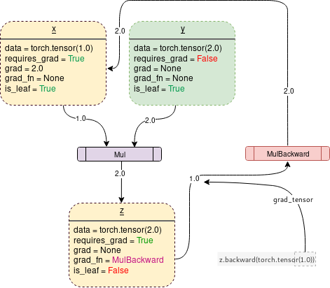
This is done in an iterative way. For each iteration, several gradients are calculated and something called a computation graph is built for storing these gradient functions. PyTorch does it by building a Dynamic Computational Graph (DCG). This graph is built from scratch in every iteration providing maximum flexibility to gradient calculation. For example, for a forward operation (function)Mul a backward operation (function) called MulBackwardis dynamically integrated in the backward graph for computing the gradient.

Dynamic Computational graph

Gradient enabled tensors (variables) along with functions (operations) combine to create the dynamic computational graph. The flow of data and the operations applied to the data are defined at runtime hence constructing the computational graph dynamically. This graph is made dynamically by the autograd class under the hood. You don’t have to encode all possible paths before you launch the training — what you run is what you differentiate.

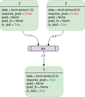
A simple DCG for multiplication of two tensors would look like this:

Each dotted outline box in the graph is a variable and the purple rectangular box is an operation.

Every variable object has several members some of which are:

Data: It’s the data a variable is holding. x holds a 1×1 tensor with the value equal to 1.0 while y holds 2.0. z holds the product of two i.e. 2.0

requires_grad: This member, if true starts tracking all the operation history and forms a backward graph for gradient calculation. For an arbitrary tensor aIt can be manipulated in-place as follows: a.requires_grad_(True).

grad: grad holds the value of gradient. If requires_grad is False it will hold a None value. Even if requires_grad is True, it will hold a None value unless .backward() function is called from some other node. For example, if you call out.backward() for some variable out that involved x in its calculations then x.grad will hold ∂out/∂x.

grad_fn: This is the backward function used to calculate the gradient.

is_leaf: A node is leaf if :

1. It was initialized explicitly by some function like x = torch.tensor(1.0) or x = torch.randn(1, 1) (basically all the tensor initializing methods discussed at the beginning of this post).
2. It is created after operations on tensors which all have requires_grad = False.
3. It is created by calling .detach() method on some tensor.

On calling backward(), gradients are populated only for the nodes which have both requires_grad and is_leaf True. Gradients are of the output node from which .backward() is called, w.r.t other leaf nodes.

On turning requires_grad = True PyTorch will start tracking the operation and store the gradient functions at each step as follows:

The code that would generate the above graph under the PyTorch’s hood is :

import torch

# Creating the graph
x = torch.tensor(1.0, requires_grad = True)
y = torch.tensor(2.0)
z = x * y

# Displaying
for i, name in zip([x, y, z], "xyz"):
    print(f"{name}\ndata: {i.data}\nrequires_grad: {i.requires_grad}\n\
grad: {i.grad}\ngrad_fn: {i.grad_fn}\nis_leaf: {i.is_leaf}\n")

In the process it never explicitly constructs the whole Jacobian. It’s usually simpler and more efficient to compute the JVP directly.

To stop PyTorch from tracking the history and forming the backward graph, the code can be wrapped inside with torch.no_grad(): It will make the code run faster whenever gradient tracking is not needed.

import torch
# Creating the graph
x = torch.tensor(1.0, requires_grad = True)
# Check if tracking is enabled
print(x.requires_grad) #True
y = x * 2
print(y.requires_grad) #True

with torch.no_grad():
	# Check if tracking is enabled
	y = x * 2
	print(y.requires_grad) #False

Backward() function

Backward is the function which actually calculates the gradient by passing it’s argument (1×1 unit tensor by default) through the backward graph all the way up to every leaf node traceable from the calling root tensor. The calculated gradients are then stored in .grad of every leaf node. Remember, the backward graph is already made dynamically during the forward pass. Backward function only calculates the gradient using the already made graph and stores them in leaf nodes.

Lets analyze the following code

import torch
# Creating the graph
x = torch.tensor(1.0, requires_grad = True)
z = x ** 3
z.backward() #Computes the gradient 
print(x.grad.data) #Prints '3' which is dz/dx 

An important thing to notice is that when z.backward() is called, a tensor is automatically passed as z.backward(torch.tensor(1.0)). The torch.tensor(1.0)is the external gradient provided to terminate the chain rule gradient multiplications. This external gradient is passed as the input to the MulBackward function to further calculate the gradient of x. The dimension of tensor passed into .backward() must be the same as the dimension of the tensor whose gradient is being calculated. For example, if the gradient enabled tensor x and y are as follows:

x = torch.tensor([0.0, 2.0, 8.0], requires_grad = True)

y = torch.tensor([5.0 , 1.0 , 7.0], requires_grad = True)

and z = x * y

then, to calculate gradients of z (a 1×3 tensor) with respect to x or y , an external gradient needs to be passed to z.backward()function as follows: z.backward(torch.FloatTensor([1.0, 1.0, 1.0])

z.backward() would give a RuntimeError: grad can be implicitly created only for scalar outputs

The tensor passed into the backward function acts like weights for a weighted output of gradient. Mathematically, this is the vector multiplied by the Jacobian matrix of non-scalar tensors (discussed further in this post) hence it should almost always be a unit tensor of dimension same as the tensor backward is called upon, unless weighted outputs needs to be calculated.

tldr : Backward graph is created automatically and dynamically by autograd class during forward pass. Backward() simply calculates the gradients by passing its argument to the already made backward graph.

Mathematics — Jacobians and vectors

Mathematically, the autograd class is just a Jacobian-vector product computing engine. A Jacobian matrix in very simple words is a matrix representing all the possible partial derivatives of two vectors. It’s the gradient of a vector with respect to another vector.

Note: In the process PyTorch never explicitly constructs the whole Jacobian. It’s usually simpler and more efficient to compute the JVP (Jacobian vector product) directly.

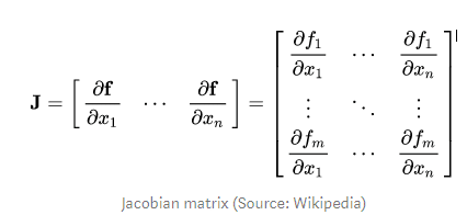
If a vector X = [x1, x2,….xn] is used to calculate some other vector f(X) = [f1, f2, …. fn] through a function f then the Jacobian matrix (J) simply contains all the partial derivative combinations as follows:

Above matrix represents the gradient of f(X)with respect to X

Suppose a PyTorch gradient enabled tensors X as:

X = [x1, x2, ….. xn] (Let this be the weights of some machine learning model)

X undergoes some operations to form a vector Y

Y = f(X) = [y1, y2, …. ym]

Y is then used to calculate a scalar loss l. Suppose a vector v happens to be the gradient of the scalar loss l with respect the vector Y as follows

To get the gradient of the loss l with respect to the weights X the Jacobian matrix J is vector-multiplied with the vector v

This method of calculating the Jacobian matrix and multiplying it with a vector v enables the possibility for PyTorch to feed external gradients with ease for even the non-scalar outputs.

[ad_2]

This article has been published from the source link without modifications to the text. Only the headline has been changed.

Source link