This article is an end-to-end example of training, testing and saving a machine learning model for image classification using the TensorFlow python package.
TensorFlow
TensorFlow is a machine learning (primarily deep learning) package developed and open-sourced by Google; when it was originally released TensorFlow was a relatively low-level package for experienced users, however in the last few years and especially since the release of TensorFlow 2.0 it is now aimed at a wider range of users.
A few years ago I ran a PoC with one of our developers that looked at running TensorFlow models offline on one of our mobile applications. Whilst we found that it was possible we also encountered a few challenges that made the solution quite fiddly. Roll forward to 2020 and TensorFlow has improved a lot; the latest version has greater integration with the Keras APIs, it’s being extended to cover more of the data processing pipeline and has also branched out to support for new languages, with the TensorFlow.js package and the use-cases that it supports being particularly interesting.
Image Classification
Image classification is one of the best known applications for deep learning, it is utilised in a range of technological developments including novelty face swapping apps, new approaches to radiology and topological analysis of the environment. Typically image classification is achieved using a special type of neural network called a convolutional neural network (CNN), this article gives a great introduction to CNNs if you want to understand a bit more about them.
Example Notebook
A corresponding Jupyter notebook can be found here.
Pre-reading
First up if you don’t have TensorFlow installed and want to follow this example, check out the install guide. The code shown here was largely taken and adapted from two image classification examples on the TensorFlow website. Firstly this basic example and secondly this one that introduces some more concepts for improving model performance.
The Data
Rather than replay a prescribed exercise from TensorFlow I wanted to use an alternative data set, I find this helps me to get more understanding of each of the steps as invariably the example code requires some alteration.
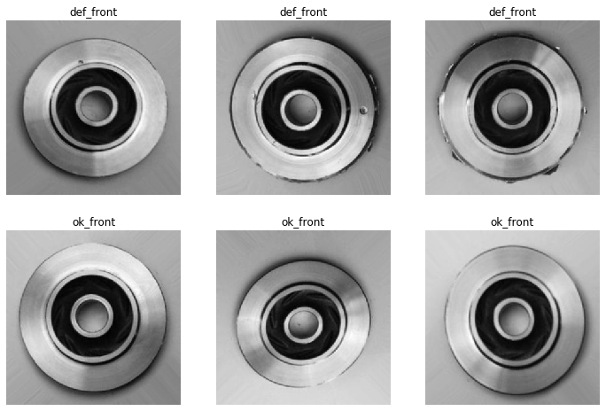
In this case I have used an open data set taken from Kaggle, containing 7348 greyscale, 300×300 pixel images of submersible pump impellers. Some of those impellers have been classified as “Ok” whilst others have been classified as “Defective”. The challenge is to train a model on that data that can be used to accurately classify images as one or the other.
Setup
Firstly import TensorFlow and confirm the version; this example was created using version 2.3.0.
import tensorflow as tf
print(tf.__version__)
Next specify some of the metadata that will be required to process the images, as mentioned these are grayscale images and so there is only 1 layer or channel of data, if these were rgb images then the number of colour layers would be 3.
color_mode = "grayscale"
number_colour_layers = 1
image_size = (300, 300)
image_shape = image_size + (number_colour_layers,)
Import & Preprocess the Data
In this case the data is already split into separate directories of training and testing data. However I want to further split the training data into a training and validation data set, for those unfamiliar with these terms the training data set is used to train the model, the validation data set it used to validate the model whilst it is training and the test set is used to assess the model once training is completed. Helpfully there is a Keras API for ingesting image data that is split into directories and this can infer the classification class names from the folder structure, all we need to do is provide the location of the data and the metadata we have already defined. Also whilst developing the code it’s nice to use a seed so that you know that changes in performance from each run are due to changes you have made rather just due to changes in the data split.
N.B Make sure to replace the data paths below with the location that you have saved the data in.
training_data_path = "./casting_data/casting_data/train"
test_data_path = "./casting_data/casting_data/test"
SEED = 42
I’m going to create a method that ingests the data and prepares it for analysis, this way I can call the method once for the training set, again for the validation set and later for the test set and know that they have been prepared in the same way.
def get_image_data(data_path, color_mode, image_size, seed = None, subset = None, validation_split = None):
    if subset:
        validation_split = 0.2
    return tf.keras.preprocessing.image_dataset_from_directory(
        data_path,
        color_mode=color_mode,
        image_size=image_size,
        seed=seed,
        validation_split=validation_split,
        subset=subset
    )
Before using this method I want to add some enhancements in, firstly to help optimise the training performance to make best use of the memory and compute available, for a deeper dive on this check out this TensorFlow performance guide.
def get_image_data(data_path, color_mode, image_size, seed = None, subset = None, validation_split = None):
    if subset:
        validation_split = 0.2
    raw_data_set = \
    tf.keras.preprocessing.image_dataset_from_directory(
        data_path,
        color_mode=color_mode,
        image_size=image_size,
        seed=seed,
        validation_split=validation_split,
        subset=subset
    )

    return raw_data_set.cache().prefetch(
        buffer_size = tf.data.experimental.AUTOTUNE
    )
Secondly I want to output the number and names of the classification classes, so I’ll alter the return type from being the FetchedDataset to being a dict containing the FetchedDataset and the list of class names.
def get_image_data(data_path, color_mode, image_size, seed = None, subset = None, validation_split = None):
    if subset:
        validation_split = 0.2
    raw_data_set = \
    tf.keras.preprocessing.image_dataset_from_directory(
        data_path,
        color_mode=color_mode,
        image_size=image_size,
        seed=seed,
        validation_split=validation_split,
        subset=subset
    )

    raw_data_set.class_names.sort()

    return {
        "data": raw_data_set.cache().prefetch(
        buffer_size = tf.data.experimental.AUTOTUNE
        ),
        "classNames": raw_data_set.class_names
    }
I can then call this method in order to create my training, validation and test data sets.
training_ds = get_image_data(
    training_data_path,
    color_mode,
    image_size,
    SEED,
    subset = "training"
)validation_ds = get_image_data(
    training_data_path,
    color_mode,
    image_size,
    SEED,
    subset = "validation"
)test_ds = get_image_data(
    test_data_path,
    color_mode,
    image_size
)
As a sanity check I just want to ensure that the name and number of classes are the same in both sets and then store the number of classes for classification to use in defining the output shape of the model.
equivalence_check = training_ds["classNames"] == validation_ds["classNames"]
assert_fail_message = "Training and Validation classes should match"
assert(equivalence_check), assert_fail_message
class_names = training_ds["classNames"]
number_classes = len(class_names)
And just whilst I’m developing the training code I want to see a small sample of the images.
from os import listdir
from os.path import join
import matplotlib.image as mpimg
import matplotlib.pyplot as plt
%matplotlib inlineimage_indexes = [286, 723, 1103]
selected_image_file_paths = dict()for classification in class_names:
    image_directory = join(training_data_path, classification)
    image_file_names = listdir(image_directory)
    selected_image_file_paths[classification] = [join(image_directory, image_file_names[i]) for i in image_indexes]plt.figure(figsize=(12, 8))

for i,classification in enumerate(class_names):
    for j,image in enumerate(selected_image_file_paths[classification]):
        image_number = (i * len(image_indexes)) + j + 1
        ax = plt.subplot(number_classes,3,image_number)
        plt.title(classification)
        plt.axis("off")
        plt.imshow(mpimg.imread(image))

Finally before starting the model construction there’s one more thing that I should consider. The grayscale channel values are in the range [0, 255] however for neural network training the values should be small, therefore I want to rescale the values to be in the range [0, 1]. Optionally I could add this in as a step in my get_image_data method, something along the lines of raw_data_set = raw_data_set / 255.0 however if I make that step part of my training data preparation then any consumer of that model (in my case some frontend code) will also have to rescale the image values in the same way…
Model Definition
Thankfully Keras now allows me to prepend the rescale operation to the start of the model which means that when it is being used later on, then the front end code can just pass it the raw image file data (providing the image is also grayscale and 300×300 pixels).
preprocessing_layers = [
    tf.keras.layers.experimental.preprocessing.Rescaling(1./255, input_shape=image_shape)
]
For the model itself I am going to deploy a common pattern using a series of convolutional layers interspersed with pooling layers.
def conv_2d_pooling_layers(filters, number_colour_layers):
    return [
        tf.keras.layers.Conv2D(
            filters,
            number_colour_layers,
            padding='same',
            activation='relu'
        ),
        tf.keras.layers.MaxPooling2D()
    ]core_layers = \
    conv_2d_pooling_layers(16, number_colour_layers) + \
    conv_2d_pooling_layers(32, number_colour_layers) + \
    conv_2d_pooling_layers(64, number_colour_layers)
To complete the model the data first needs to be unwound to 1D and then dense layers deployed to ensure the output has number of nodes equal to the number of possible classifications.
dense_layers = [
    tf.keras.layers.Flatten(),
    tf.keras.layers.Dense(128, activation='relu'),
    tf.keras.layers.Dense(number_classes)
]
I can then put all of these layers together in a sequential model.
model = tf.keras.Sequential(
    preprocessing_layers +
    core_layers +
    dense_layers
)
And then just define the compilation options for the model.
loss = tf.keras.losses.SparseCategoricalCrossentropy(from_logits=True)
model.compile(
    optimizer='adam',
    loss=loss,
    metrics=['accuracy']
)
Training the Model
I’m setting the max number of epochs at 20 but in order to guard against overfitting I am going to set the training to stop when it detects that validation loss is no longer improving.
callback = tf.keras.callbacks.EarlyStopping(
    monitor='val_loss', min_delta=0, patience=3, verbose=0, mode='auto',
    baseline=None, restore_best_weights=True
)history = model.fit(
    training_ds["data"],
    validation_data = validation_ds["data"],
    epochs = 20,
    callbacks = [callback]
)
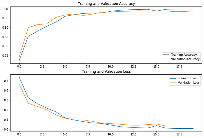
At the end of 20 epochs the model training has finished and the accuracy is very high (between 98% and 99%), this is more likely due to careful control of the conditions in which the data was captured or some augmentation of the images rather than the model itself being particularly good, as it has not been optimised. Often in real world scenarios, variability in the data makes it difficult to train accurate models without careful preprocessing of the images themselves (normalising for lighting, background, device quality, shot angle, shot distance etc.).
Evaluate the Model & Training
Having trained the model the next step is to test it, we can do this by calling the evaluate method and passing it the test data.
model.evaluate(test_ds["data"])
In this instance the model performs very well in testing (99% accuracy) as well as training, in some cases though you may find that a model achieves high accuracy in training but then performs poorly in testing; this could be due to overfitting but in our case we have taken steps to guard against overfitting or it could be that the testing and training data set are taken from different distributions, one approach to investigating this would be to combine, shuffle and re-split the data sets.
We can also plot the performance of the model during training, below we can see that the accuracy and loss improved relatively steadily and then started to plateau when the accuracy got very high (as you would expect), however there were epochs where performance worsened, with a lower patience setting the training would have stopped at those points.
acc = history.history['accuracy']
val_acc = history.history['val_accuracy']loss = history.history['loss']
val_loss = history.history['val_loss']epochs_range = range(len(acc))plt.figure(figsize=(12, 8))
plt.subplot(2, 1, 1)
plt.plot(epochs_range, acc, label='Training Accuracy')
plt.plot(epochs_range, val_acc, label='Validation Accuracy')
plt.legend(loc='lower right')
plt.title('Training and Validation Accuracy')plt.subplot(2, 1, 2)
plt.plot(epochs_range, loss, label='Training Loss')
plt.plot(epochs_range, val_loss, label='Validation Loss')
plt.legend(loc='upper right')
plt.title('Training and Validation Loss')
plt.show()

Saving the Model
Because my use-case is for usage with TensorFlow.js I am going to save the model in the format required by TensorFlow.js rather than the usual formats. To do that I will need to install another package.
import tensorflowjs as tfjstfjs.converters.save_keras_model(
    model,
    "./tmp/model_js_1"
)
Once it is in this format I can share it with frontend developers, who can then potentially create an application for loading and classifying images in an online or offline scenario.
Conclusion
Improvements to TensorFlow over the last few years mean it’s easier to work with for those who are looking to get started with training and deploying deep learning models, there’s also great documentation online so it’d definitely worth looking at. I’ve tried to make this code easy to work with if you want to adapt it to your own use-cases or data-sets and I think that’s a great way to learn as it forces you to look a bit more closely at each stage.
This article has been published from the source link without modifications to the text. Only the headline has been changed.
Source link


