What are Decision Trees?

In simple words, a decision tree is a structure that contains nodes (rectangular boxes) and edges(arrows) and is built from a dataset (table of columns representing features/attributes and rows corresponds to records). Each node is either used to make a decision (known as decision node) or represent an outcome (known as leaf node).

Decision tree Example

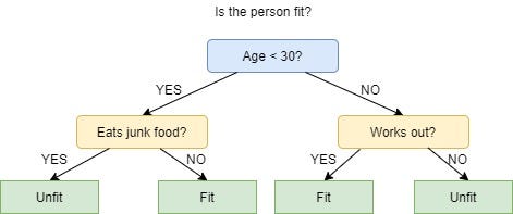
The picture above depicts a decision tree that is used to classify whether a person is Fit or Unfit.
The decision nodes here are questions like ‘’‘Is the person less than 30 years of age?’, ‘Does the person eat junk?’, etc. and the leaves are one of the two possible outcomes viz. Fit and Unfit.
Looking at the Decision Tree we can say make the following decisions:
if a person is less than 30 years of age and doesn’t eat junk food then he is Fit, if a person is less than 30 years of age and eats junk food then he is Unfit and so on.

The initial node is called the root node (colored in blue), the final nodes are called the leaf nodes (colored in green) and the rest of the nodes are called intermediate or internal nodes.
The root and intermediate nodes represent the decisions while the leaf nodes represent the outcomes.

ID3 in brief

ID3 stands for Iterative Dichotomiser 3 and is named such because the algorithm iteratively (repeatedly) dichotomizes(divides) features into two or more groups at each step.

Invented by Ross Quinlan, ID3 uses a top-down greedy approach to build a decision tree. In simple words, the top-down approach means that we start building the tree from the top and the greedy approach means that at each iteration we select the best feature at the present moment to create a node.

Most generally ID3 is only used for classification problems with nominal features only.

Dataset description

In this article, we’ll be using a sample dataset of COVID-19 infection. A preview of the entire dataset is shown below.

+----+-------+-------+------------------+----------+
| ID | Fever | Cough | Breathing issues | Infected |
+----+-------+-------+------------------+----------+
| 1  | NO    | NO    | NO               | NO       |
+----+-------+-------+------------------+----------+
| 2  | YES   | YES   | YES              | YES      |
+----+-------+-------+------------------+----------+
| 3  | YES   | YES   | NO               | NO       |
+----+-------+-------+------------------+----------+
| 4  | YES   | NO    | YES              | YES      |
+----+-------+-------+------------------+----------+
| 5  | YES   | YES   | YES              | YES      |
+----+-------+-------+------------------+----------+
| 6  | NO    | YES   | NO               | NO       |
+----+-------+-------+------------------+----------+
| 7  | YES   | NO    | YES              | YES      |
+----+-------+-------+------------------+----------+
| 8  | YES   | NO    | YES              | YES      |
+----+-------+-------+------------------+----------+
| 9  | NO    | YES   | YES              | YES      |
+----+-------+-------+------------------+----------+
| 10 | YES   | YES   | NO               | YES      |
+----+-------+-------+------------------+----------+
| 11 | NO    | YES   | NO               | NO       |
+----+-------+-------+------------------+----------+
| 12 | NO    | YES   | YES              | YES      |
+----+-------+-------+------------------+----------+
| 13 | NO    | YES   | YES              | NO       |
+----+-------+-------+------------------+----------+
| 14 | YES   | YES   | NO               | NO       |
+----+-------+-------+------------------+----------+

The columns are self-explanatory. Y and N stand for Yes and No respectively. The values or classes in Infected column Y and N represent Infected and Not Infected respectively.

The columns used to make decision nodes viz. ‘Breathing Issues’, ‘Cough’ and ‘Fever’ are called feature columns or just features and the column used for leaf nodes i.e. ‘Infected’ is called the target column.

Metrics in ID3

As mentioned previously, the ID3 algorithm selects the best feature at each step while building a Decision tree.
Before you ask, the answer to the question: ‘How does ID3 select the best feature?’ is that ID3 uses Information Gain or just Gain to find the best feature.

Information Gain calculates the reduction in the entropy and measures how well a given feature separates or classifies the target classes. The feature with the highest Information Gain is selected as the best one.

In simple words, Entropy is the measure of disorder and the Entropy of a dataset is the measure of disorder in the target feature of the dataset.
In the case of binary classification (where the target column has only two types of classes) entropy is 0 if all values in the target column are homogenous(similar) and will be 1 if the target column has equal number values for both the classes.

We denote our dataset as S, entropy is calculated as:

Entropy(S) = - ∑ pᵢ * log₂(pᵢ) ; i = 1 to n

where,
n is the total number of classes in the target column (in our case n = 2 i.e YES and NO)
pᵢ is the probability of class ‘i’ or the ratio of “number of rows with class i in the target column” to the “total number of rows” in the dataset.

Information Gain for a feature column A is calculated as:

IG(S, A) = Entropy(S) - ∑((|Sᵥ| / |S|) * Entropy(Sᵥ))

where Sᵥ is the set of rows in S for which the feature column A has value v, |Sᵥ| is the number of rows in Sᵥ and likewise |S| is the number of rows in S.

ID3 Steps

1. Calculate the Information Gain of each feature.
2. Considering that all rows don’t belong to the same class, split the dataset S into subsets using the feature for which the Information Gain is maximum.
3. Make a decision tree node using the feature with the maximum Information gain.
4. If all rows belong to the same class, make the current node as a leaf node with the class as its label.
5. Repeat for the remaining features until we run out of all features, or the decision tree has all leaf nodes.

Implementation on our Dataset

As stated in the previous section the first step is to find the best feature i.e. the one that has the maximum Information Gain(IG). We’ll calculate the IG for each of the features now, but for that, we first need to calculate the entropy of S

From the total of 14 rows in our dataset S, there are 8 rows with the target value YES and 6 rows with the target value NO. The entropy of S is calculated as:

Entropy(S) = — (8/14) * log₂(8/14) — (6/14) * log₂(6/14) = 0.99

Note: If all the values in our target column are same the entropy will be zero (meaning that it has no or zero randomness).

We now calculate the Information Gain for each feature:

IG calculation for Fever:
In this(Fever) feature there are 8 rows having value YES and 6 rows having value NO.
As shown below, in the 8 rows with YES for Fever, there are 6 rows having target value YES and 2 rows having target value NO.

+-------+-------+------------------+----------+
| Fever | Cough | Breathing issues | Infected |
+-------+-------+------------------+----------+
| YES   | YES   | YES              | YES      |
+-------+-------+------------------+----------+
| YES   | YES   | NO               | NO       |
+-------+-------+------------------+----------+
| YES   | NO    | YES              | YES      |
+-------+-------+------------------+----------+
| YES   | YES   | YES              | YES      |
+-------+-------+------------------+----------+
| YES   | NO    | YES              | YES      |
+-------+-------+------------------+----------+
| YES   | NO    | YES              | YES      |
+-------+-------+------------------+----------+
| YES   | YES   | NO               | YES      |
+-------+-------+------------------+----------+
| YES   | YES   | NO               | NO       |
+-------+-------+------------------+----------+

As shown below, in the 6 rows with NO, there are 2 rows having target value YES and 4 rows having target value NO.

+-------+-------+------------------+----------+
| Fever | Cough | Breathing issues | Infected |
+-------+-------+------------------+----------+
| NO    | NO    | NO               | NO       |
+-------+-------+------------------+----------+
| NO    | YES   | NO               | NO       |
+-------+-------+------------------+----------+
| NO    | YES   | YES              | YES      |
+-------+-------+------------------+----------+
| NO    | YES   | NO               | NO       |
+-------+-------+------------------+----------+
| NO    | YES   | YES              | YES      |
+-------+-------+------------------+----------+
| NO    | YES   | YES              | NO       |
+-------+-------+------------------+----------+

The block, below, demonstrates the calculation of Information Gain for Fever.

# total rows
|S| = 14For v = YES, |Sᵥ| = 8
Entropy(Sᵥ) = - (6/8) * log₂(6/8) - (2/8) * log₂(2/8) = 0.81For v = NO, |Sᵥ| = 6
Entropy(Sᵥ) = - (2/6) * log₂(2/6) - (4/6) * log₂(4/6) = 0.91# Expanding the summation in the IG formula:
IG(S, Fever) = Entropy(S) - (|Sʏᴇꜱ| / |S|) * Entropy(Sʏᴇꜱ) - 
(|Sɴᴏ| / |S|) * Entropy(Sɴᴏ)∴ IG(S, Fever) = 0.99 - (8/14) * 0.81 - (6/14) * 0.91 = 0.13

Next, we calculate the IG for the features “Cough” and “Breathing issues”.
You can use this free online tool to calculate the Information Gain.

IG(S, Cough) = 0.04
IG(S, BreathingIssues) = 0.40

Since the feature Breathing issues have the highest Information Gain it is used to create the root node.
Hence, after this initial step our tree looks like this:

Next, from the remaining two unused features, namely, Fever and Cough, we decide which one is the best for the left branch of Breathing Issues.
Since the left branch of Breathing Issues denotes YES, we will work with the subset of the original data i.e the set of rows having YES as the value in the Breathing Issues column. These 8 rows are shown below:

+-------+-------+------------------+----------+
| Fever | Cough | Breathing issues | Infected |
+-------+-------+------------------+----------+
| YES   | YES   | YES              | YES      |
+-------+-------+------------------+----------+
| YES   | NO    | YES              | YES      |
+-------+-------+------------------+----------+
| YES   | YES   | YES              | YES      |
+-------+-------+------------------+----------+
| YES   | NO    | YES              | YES      |
+-------+-------+------------------+----------+
| YES   | NO    | YES              | YES      |
+-------+-------+------------------+----------+
| NO    | YES   | YES              | YES      |
+-------+-------+------------------+----------+
| NO    | YES   | YES              | YES      |
+-------+-------+------------------+----------+
| NO    | YES   | YES              | NO       |
+-------+-------+------------------+----------+

Next, we calculate the IG for the features Fever and Cough using the subset Sʙʏ (Set Breathing Issues Yes) which is shown above :

Note: For IG calculation the Entropy will be calculated from the subset Sʙʏ and not the original dataset S.

IG(Sʙʏ, Fever) = 0.20
IG(Sʙʏ, Cough) = 0.09

IG of Fever is greater than that of Cough, so we select Fever as the left branch of Breathing Issues:
Our tree now looks like this:

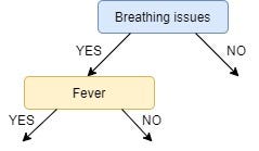
Next, we find the feature with the maximum IG for the right branch of Breathing Issues. But, since there is only one unused feature left we have no other choice but to make it the right branch of the root node.
So our tree now looks like this:

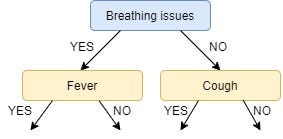
There are no more unused features, so we stop here and jump to the final step of creating the leaf nodes.
For the left leaf node of Fever, we see the subset of rows from the original data set that has Breathing Issues and Fever both values as YES.

+-------+-------+------------------+----------+
| Fever | Cough | Breathing issues | Infected |
+-------+-------+------------------+----------+
| YES   | YES   | YES              | YES      |
+-------+-------+------------------+----------+
| YES   | NO    | YES              | YES      |
+-------+-------+------------------+----------+
| YES   | YES   | YES              | YES      |
+-------+-------+------------------+----------+
| YES   | NO    | YES              | YES      |
+-------+-------+------------------+----------+
| YES   | NO    | YES              | YES      |
+-------+-------+------------------+----------+

Since all the values in the target column are YES, we label the left leaf node as YES, but to make it more logical we label it Infected.

Similarly, for the right node of Fever we see the subset of rows from the original data set that have Breathing Issues value as YES and Fever as NO.

+-------+-------+------------------+----------+
| Fever | Cough | Breathing issues | Infected |
+-------+-------+------------------+----------+
| NO    | YES   | YES              | YES      |
+-------+-------+------------------+----------+
| NO    | YES   | YES              | NO       |
+-------+-------+------------------+----------+
| NO    | YES   | YES              | NO       |
+-------+-------+------------------+----------+

Here not all but most of the values are NO, hence NO or Not Infected becomes our right leaf node.
Our tree, now, looks like this:

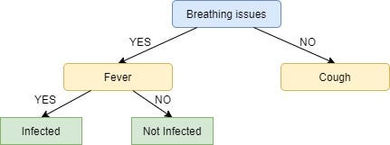
We repeat the same process for the node Cough, however here both left and right leaves turn out to be the same i.e. NO or Not Infected as shown below:

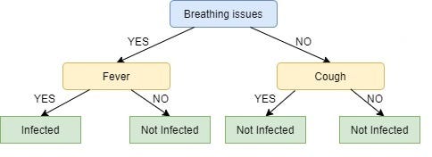
Looks Strange, doesn’t it?
I know! The right node of Breathing issues is as good as just a leaf node with class ‘Not infected’. This is one of the Drawbacks of ID3, it doesn’t do pruning.

Pruning is a mechanism that reduces the size and complexity of a Decision tree by removing unnecessary nodes. More about pruning can be found here.

Another drawback of ID3 is overfitting or high variance i.e. it learns the dataset it used so well that it fails to generalize on new data.

Summary

We covered the process of the ID3 algorithm in detail and saw how easy it was to create a Decision Tree using this algorithm by using only two metrics viz. Entropy and Information Gain.

This article has been published from the source link without modifications to the text. Only the headline has been changed.

Source link