[ad_1]
In this article, we will discuss why we need batch normalization and dropout in deep neural networks followed by experiments using Pytorch on a standard data set to see the effects of batch normalization and dropout. This article is based on my understanding of deep learning lectures from PadhAI.
Citation Note: The content and the structure of this article is based on the deep learning lectures from One-Fourth Labs — PadhAI.
Why Normalize Inputs?
Before we discuss batch normalization, we will learn about why normalizing the inputs speed up the training of a neural network.
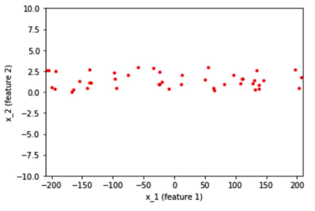
Consider a scenario where we have 2D data with features x_1 and x_2 going into a neural network. One of these features x_1 has a wider spread from -200 to 200 and another feature x_2 has a narrower spread from -10 to 10.
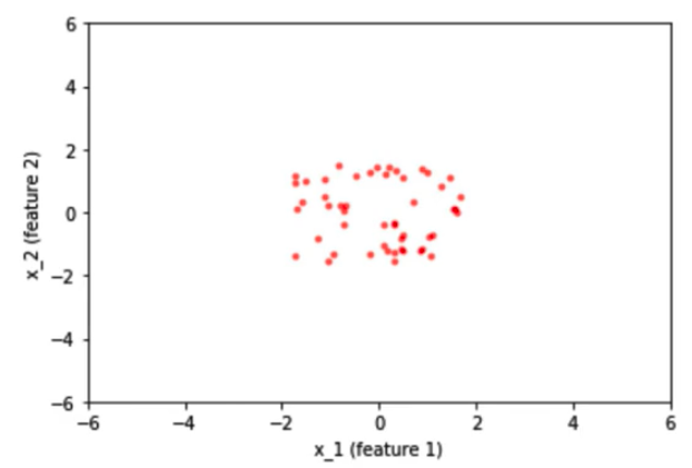
Once we normalized the data, the spread of the data for both the features is concentrated in one region ie… from -2 to 2. Spread would look like this,
Let’s discuss why normalizing inputs help?
Before we normalized the inputs, the weights associated with these inputs would vary a lot because the input features present in different ranges varying from -200 to 200 and from -2 to 2. To accommodate this range difference between the features some weights would have to be large and then some have to be small. If we have larger weights then the updates associated with the back-propagation would also be large and vice versa. Because of this uneven distribution of weights for the inputs, the learning algorithm keeps oscillating in the plateau region before it finds the global minima.
To avoid the learning algorithm spend much time oscillating in the plateau, we normalize the input features such that all the features would be on the same scale. Since our inputs are on the same scale, the weights associated with them would also be on the same scale. Thus helping the network to train faster.
Batch Normalization
We have normalized the inputs but what about hidden representatives?
By normalizing the inputs we are able to bring all the inputs features to the same scale. In the neural network, we need to compute the pre-activation for the first neuron of the first layer a₁₁. We know that pre-activation is nothing but the weighted sum of inputs plus bias. In other words, it is the dot product between the first row of the weight matrix W₁ and the input matrix X plus bias b₁₁.
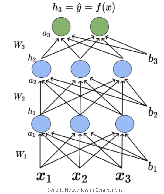
The mathematical equation for pre-activation at each layer ‘i’ is given by,

The activation at each layer is equal to applying the activation function to the output of the pre-activation of that layer. The mathematical equation for the activation at each layer ‘i’ is given by,

Similarly, the activation values for ‘n’ number of hidden layers present in the network need to be computed. The activation values will act as an input to the next hidden layers present in the network. so it doesn’t matter what we have done to the input whether we normalized them or not, the activation values would vary a lot as we do deeper and deeper into the network based on the weight associated with the corresponding neuron.
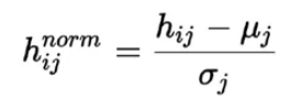
In order to bring all the activation values to the same scale, we normalize the activation values such that the hidden representation doesn’t vary drastically and also helps us to get improvement in the training speed.
Why is it called batch normalization?
Since we are computing the mean and standard deviation from a single batch as opposed to computing it from the entire data. Batch normalization is done individually at each hidden neuron in the network.
Learning Gamma γ and Beta β
Since we are normalizing all the activations in the network, are we enforcing some constraints that could deteriorate the performance of the network?
In order to maintain the representative power of the hidden neural network, batch normalization introduces two extra parameters — Gamma and Beta. Once we normalize the activation, we need to perform one more step to get the final activation value that can be feed as the input to another layer.
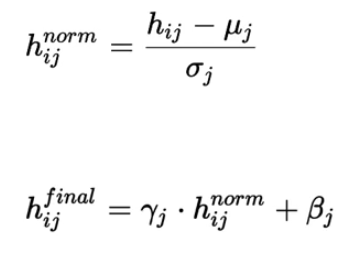
The parameters Gamma and Beta are learned along with other parameters of the network. If Gamma (γ) is equal to the mean (μ) and Beta (β) is equal to the standard deviation(σ) then the activation h_final is equal to the h_norm, thus preserving the representative power of the network.
Run this notebook in Colab
All the code discussed in the article is present on my GitHub. You can open the code notebook with any setup by directly opening my Jupyter Notebook on Github with Colab which runs on Google’s Virtual Machine. Click here, if you just want to quickly open the notebook and follow along with this tutorial.Niranjankumar-c/DeepLearning-PadhAIAll the code files related to the deep learning course from PadhAI – Niranjankumar-c/DeepLearning-PadhAIgithub.com
Batch Normalization Using Pytorch
To see how batch normalization works we will build a neural network using Pytorch and test it on the MNIST data set.

Batch Normalization — 1D
In this section, we will build a fully connected neural network (DNN) to classify the MNIST data instead of using CNN. The main purpose of using DNN is to explain how batch normalization works in case of 1D input like an array. Before we feed the MNIST images of size 28×28 to the network, we flatten them into a one-dimensional input array of size 784.
class MyNet(nn.Module):
    def __init__(self):
        super(MyNet, self).__init__()
        self.classifier = nn.Sequential(
            nn.Linear(784, 48),  # 28 x 28 = 784 flatten the input image
            nn.ReLU(),
            nn.Linear(48, 24),
            nn.ReLU(),
            nn.Linear(24, 10)
        )

    def forward(self, x):
        x = x.view(x.size(0), -1)
        x = self.classifier(x)
        return x

class MyNetBN(nn.Module):
    def __init__(self):
        super(MyNetBN, self).__init__()
        self.classifier = nn.Sequential(
            nn.Linear(784, 48),
            nn.BatchNorm1d(48), #applying batch norm
            nn.ReLU(),
            nn.Linear(48, 24),
            nn.BatchNorm1d(24),
            nn.ReLU(),
            nn.Linear(24, 10)
        )

    def forward(self, x):
        x = x.view(x.size(0), -1)
        x = self.classifier(x)
        return x
We will create two deep neural networks with three fully connected linear layers and alternating ReLU activation in between them. In the case of network with batch normalization, we will apply batch normalization before ReLU as provided in the original paper. Since our input is a 1D array we will use BatchNorm1d class present in the Pytorch nn module.
import torch.nn as nn
nn.BatchNorm1d(48) #48 corresponds to the number of input features it is getting from the previous layer.
To get a better insight into how batch normalization helps in faster converge of the network, we will look at the distribution of values across multiple hidden layers in the network during the training phase.
For consistency, we will plot the output of the second linear layer from the two networks and compare the distributions of the output from that layer across the networks. The results look like this:
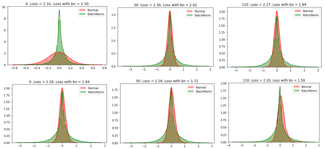
From the graphs, we can conclude that the distribution of values without batch normalization has changed significantly between iterations of inputs within each epoch which means that the subsequent layers in the network without batch normalization are seeing a varying distribution of input data. But the change in the distribution of values for the model with batch normalization seems to be slightly negligible.
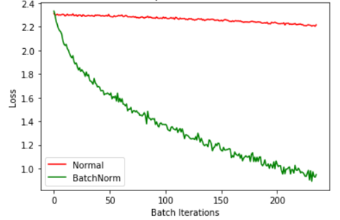
Also, we can see that the loss of the network with batch normalization reduces much faster than the normal network because of the covariance shift i.e…shifting of hidden values for each batch of input. This helps in faster converge of the network and reduces the training time.
Batch Normalization — 2D
In the previous section, we have seen how to write batch normalization between linear layers for feed-forward neural networks which take a 1D array as an input. In this section, we will discuss how to implement batch normalization for Convolution Neural Networks from a syntactical point of view.
class CNN_BN(nn.Module):
    def __init__(self):
        super(MyNetBN, self).__init__()
        self.features = nn.Sequential(
            nn.Conv2d(1, 3, 5),         # (N, 1, 28, 28) -> (N,  3, 24, 24)
            nn.ReLU(),
            nn.AvgPool2d(2, stride=2),  # (N, 3, 24, 24) -> (N,  3, 12, 12)
            nn.Conv2d(3, 6, 3),
            nn.BatchNorm2d(6)           # (N, 3, 12, 12) -> (N,  6, 10, 10)
        )
        self.features1 = nn.Sequential(
            nn.ReLU(),
            nn.AvgPool2d(2, stride=2)   # (N, 6, 10, 10) -> (N,  6, 5, 5)
        )
        self.classifier = nn.Sequential(
            nn.Linear(150, 25),         # (N, 150) -> (N, 25)
            nn.ReLU(),
            nn.Linear(25,10)            # (N, 25) -> (N, 10)
        )

    def forward(self, x):
        x = self.features(x)
        x = self.features1(x)
        x = x.view(x.size(0), -1)
        x = self.classifier(x)
        return x
We will take the same MNIST data images and write a network that implements batch normalization. The batch of RGB images has four dimensions — batch_size x channels x height x width. In the case of images, we normalize the batch over each channel. The class BatchNorm2d applies batch normalization over a 4D input (a mini-batch of 2D inputs with additional channel dimension).
The class BatchNorm2d takes the number of channels it receives from the output of a previous layer as a parameter.
Dropout
In this section of the article, we discuss the concept of dropout in neural networks specifically how it helps to reduce overfitting and generalization error. After that, we will implement a neural network with and without dropout to see how dropout influences the performance of a network using Pytorch.
Dropout is a regularization technique that “drops out” or “deactivates” few neurons in the neural network randomly in order to avoid the problem of overfitting.
The idea of Dropout
Training one deep neural network with large parameters on the data might lead to overfitting. Can we train multiple neural networks with different configurations on the same dataset and take the average value of these predictions?.
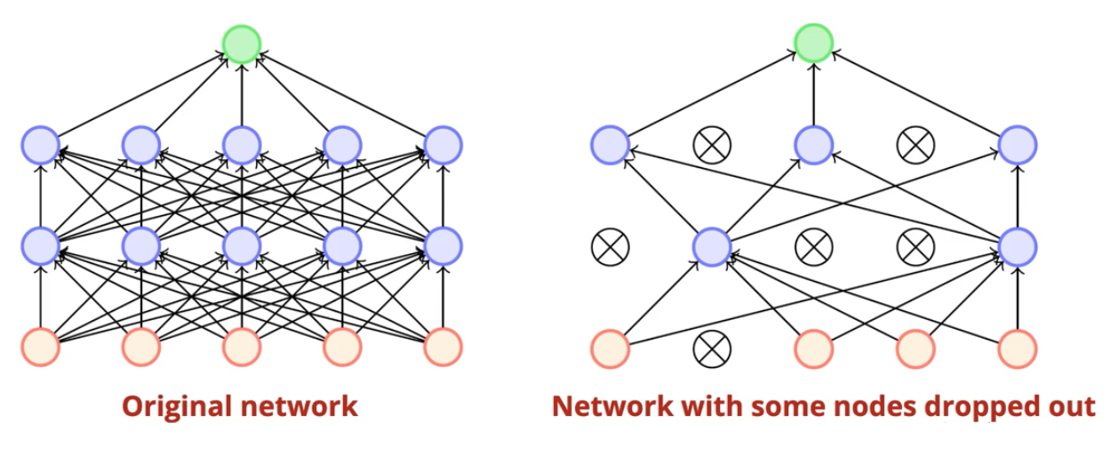
But creating an ensemble of neural networks with different architectures and training them wouldn’t be feasible in practice. Dropout to the rescue.
Dropout deactivates the neurons randomly at each training step instead of training the data on the original network, we train the data on the network with dropped out nodes. In the next iteration of the training step, the hidden neurons which are deactivated by dropout changes because of its probabilistic behavior. In this way, by applying dropout i.e…deactivating certain individual nodes at random during training we can simulate an ensemble of neural network with different architectures.
Dropout at Training time
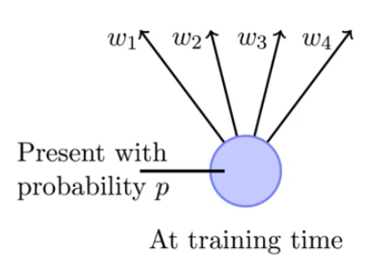
In each training iteration, each node in the network is associated with a probability p whether to keep in the network or to deactivate it (dropout) out of the network with probability 1-p. That means the weights associated with the nodes got updated only p fraction of times because nodes are active only p times during training.
Dropout at Test time
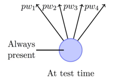
During test time, we consider the original neural network with all activations present and scale the output of each node by a value p. Since each node is activated the only p times.
Dropout Using Pytorch
To visualize how dropout reduces the overfitting of a neural network, we will generate a simple random data points using Pytorch torch.unsqueeze. The utility of the dropout is best shown on custom data that has the potential to overfit.
N = 50 #number of data points
noise = 0.3

#generate the train data
X_train = torch.unsqueeze(torch.linspace(-1, 1, N),1)
Y_train = X_train + noise * torch.normal(torch.zeros(N,1), torch.ones(N,1))

#generate the test data
X_test = torch.unsqueeze(torch.linspace(-1,1,N),1)
Y_test = X_test + noise * torch.normal(torch.zeros(N,1), torch.ones(N,1))
Once we generate the data, we can visualize the tensors using matplotlib scatter plot as shown below.
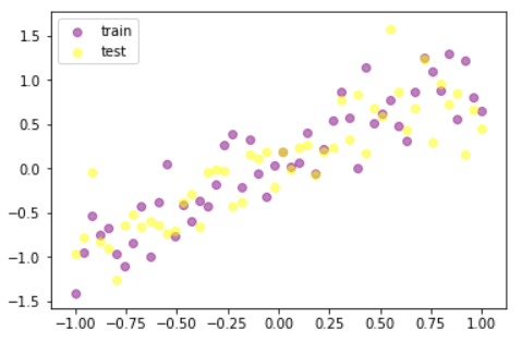
To show the overfitting, we will train two networks — one without dropout and another with dropout. The network without dropout has 3 fully connected hidden layers with ReLU as the activation function for the hidden layers and the network with dropout also has similar architecture but with dropout applied after first & second Linear layer.
#create a neural network with out dropout
N_h = 100 #hidden nodes

model = torch.nn.Sequential(
    nn.Linear(1, N_h),
    nn.ReLU(),
    nn.Linear(N_h, N_h),
    nn.ReLU(),
    nn.Linear(N_h, 1)
)

#create a network with dropout
model_dropout = nn.Sequential(
    nn.Linear(1, N_h),
    nn.Dropout(0.5), #50 % probability
    nn.ReLU(),
    torch.nn.Linear(N_h, N_h),
    torch.nn.Dropout(0.2), #20% probability
    torch.nn.ReLU(),
    torch.nn.Linear(N_h, 1),
)
In Pytorch, we can apply a dropout using torch.nn module.
import torch.nn as nn
nn.Dropout(0.5) #apply dropout in a neural network
In this example, I have used a dropout fraction of 0.5 after the first linear layer and 0.2 after the second linear layer. Once we train the two different models i.e…one without dropout and another with dropout and plot the test results, it would look like this:
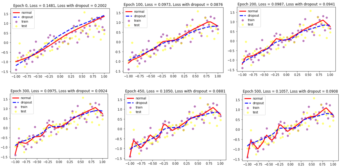
From the above graphs, we can conclude that as we increase the number of epochs the model without dropout is overfitting the data. The model without dropout is learning the noise associated with the data instead of generalizing for the data. We can see that the loss associated with the model without drop increases as we increase the number of epochs unlike the loss associated with the model with dropout.Niranjankumar-c/DeepLearning-PadhAIAll the code files related to the deep learning course from PadhAI – Niranjankumar-c/DeepLearning-PadhAIgithub.com
Conclusion
In this article, we have discussed why we need batch normalization and then we went on to visualize the effect of batch normalization on the outputs of hidden layers using the MNIST data set. After that, we discussed the working of dropout and it prevents the problem of overfitting the data. Finally, we visualized the performance of two networks with and without dropout to see the effect of dropout.
[ad_2]
This article has been published from the source link without modifications to the text. Only the headline has been changed.


