One of the most well-liked methods for training deep neural networks is the gradient descent algorithm. It has numerous uses in areas including speech recognition, computer vision, and natural language processing. Although the concept of gradient descent has been around for a long time, it has only lately been used in deep learning applications.
Gradient descent is an iterative optimization technique that updates values repeatedly at each step to determine the minimum of an objective function. It moves incrementally in the desired direction with each iteration until convergence or a stop condition is attained.
In this tutorial, you will learn how to use PyTorch to create gradient descent and train a straightforward linear regression model with two trainable parameters. You’ll discover more specifically about:
- The Gradient Descent technique and PyTorch’s implementation
- Batch Gradient Descent and PyTorch’s use of it
- Stochastic Gradient Descent and PyTorch’s use of it
- What distinguishes Stochastic Gradient Descent from Batch Gradient Descent
- How loss diminishes during training in batch gradient descent versus stochastic gradient descent
So let’s get going.
Overview
There are four sections to this tutorial.
- Data Preparation
- Batch Gradient Descent
- Stochastic Gradient Descent
- Plotting Graphs for Comparison
Data Preparation
We will take a linear regression example to illustrate how to keep the model basic. The data is fabricated and produced as follows:
import torch
import numpy as np
import matplotlib.pyplot as plt

# Creating a function f(X) with a slope of -5
X = torch.arange(-5, 5, 0.1).view(-1, 1)
func = -5 * X

# Adding Gaussian noise to the function f(X) and saving it in Y
Y = func + 0.4 * torch.randn(X.size())
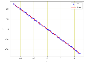
Similarly to the prior tutorial, we set up a variable called X with values ranging from −5 to 5, and generated a linear function with a slope of −5. Next, a Gaussian noise component is introduced to produce the variable Y.
Using Matplotlib, we can plot the data to show the pattern:
...
# Plot and visualizing the data points in blue
plt.plot(X.numpy(), Y.numpy(), 'b+', label='Y')
plt.plot(X.numpy(), func.numpy(), 'r', label='func')
plt.xlabel('x')
plt.ylabel('y')
plt.legend()
plt.grid('True', color='y')
plt.show()
Data points for regression model
Batch Gradient Descent
Following the creation of the model’s data, we will construct a forward function based on a straightforward linear regression equation. We will train the model using the two parameters (w and b). Moreover, a loss criterion function is required. MSE loss is appropriate because it is a regression problem on continuous values.
...
# defining the function for forward pass for prediction
def forward(x):
return w * x + b

# evaluating data points with Mean Square Error (MSE)
def criterion(y_pred, y):
return torch.mean((y_pred - y) ** 2)
Learn more about batch gradient descent before we train our model. All of the samples in the training data are taken into account at once when using batch gradient descent. By using the mean gradient of all the training examples, the parameters are updated. Therefore, there is just one gradient descent step in one epoch.
Even though Batch Gradient Descent is the best option for smooth error manifolds, it is comparatively sluggish and computationally challenging, especially if you need to train on a bigger dataset.
Training with Batch Gradient Descent
Let’s randomize the initialization of the training parameters w and b, and let’s establish some training parameters, such as learning rate or step size, an empty list to store the loss, and the number of training epochs.
w = torch.tensor(-10.0, requires_grad=True)
b = torch.tensor(-20.0, requires_grad=True)

step_size = 0.1
loss_BGD = []
n_iter = 20
The code below will be used to train our model for 20 epochs. While the criterion() method assesses the loss and stores it in the loss variable, the forward() function creates the prediction in this case. The gradient calculations are carried out via the backward() method and the modified parameters are saved in the w.data and b.data.
for i in range (n_iter):
# making predictions with forward pass
Y_pred = forward(X)
# calculating the loss between original and predicted data points
loss = criterion(Y_pred, Y)
# storing the calculated loss in a list
loss_BGD.append(loss.item())
# backward pass for computing the gradients of the loss w.r.t to learnable parameters
loss.backward()
# updateing the parameters after each iteration
w.data = w.data - step_size * w.grad.data
b.data = b.data - step_size * b.grad.data
# zeroing gradients after each iteration
w.grad.data.zero_()
b.grad.data.zero_()
# priting the values for understanding
print('{}, \t{}, \t{}, \t{}'.format(i, loss.item(), w.item(), b.item()))
Here is an example of the result from applying batch gradient descent, where the parameters are updated after each epoch.
0, 596.7191162109375, -1.8527469635009766, -16.062074661254883
1, 343.426513671875, -7.247585773468018, -12.83026123046875
2, 202.7098388671875, -3.616910219192505, -10.298759460449219
3, 122.16651153564453, -6.0132551193237305, -8.237251281738281
4, 74.85094451904297, -4.394278526306152, -6.6120076179504395
5, 46.450958251953125, -5.457883358001709, -5.295622825622559
6, 29.111614227294922, -4.735295295715332, -4.2531514167785645
7, 18.386211395263672, -5.206836700439453, -3.4119482040405273
8, 11.687058448791504, -4.883906364440918, -2.7437009811401367
9, 7.4728569984436035, -5.092618465423584, -2.205873966217041
10, 4.808231830596924, -4.948029518127441, -1.777699589729309
11, 3.1172332763671875, -5.040188312530518, -1.4337140321731567
12, 2.0413269996643066, -4.975278854370117, -1.159447193145752
13, 1.355530858039856, -5.0158305168151855, -0.9393846988677979
14, 0.9178376793861389, -4.986582279205322, -0.7637402415275574
15, 0.6382412910461426, -5.004333972930908, -0.6229321360588074
16, 0.45952412486076355, -4.991086006164551, -0.5104631781578064
17, 0.34523946046829224, -4.998797416687012, -0.42035552859306335
18, 0.27213525772094727, -4.992753028869629, -0.3483465909957886
19, 0.22536347806453705, -4.996064186096191, -0.2906789183616638
Here is the full code after it has been put all together.
import torch
import numpy as np
import matplotlib.pyplot as plt

X = torch.arange(-5, 5, 0.1).view(-1, 1)
func = -5 * X
Y = func + 0.4 * torch.randn(X.size())

# defining the function for forward pass for prediction
def forward(x):
return w * x + b

# evaluating data points with Mean Square Error (MSE)
def criterion(y_pred, y):
return torch.mean((y_pred - y) ** 2)

w = torch.tensor(-10.0, requires_grad=True)
b = torch.tensor(-20.0, requires_grad=True)

step_size = 0.1
loss_BGD = []
n_iter = 20

for i in range (n_iter):
# making predictions with forward pass
Y_pred = forward(X)
# calculating the loss between original and predicted data points
loss = criterion(Y_pred, Y)
# storing the calculated loss in a list
loss_BGD.append(loss.item())
# backward pass for computing the gradients of the loss w.r.t to learnable parameters
loss.backward()
# updateing the parameters after each iteration
w.data = w.data - step_size * w.grad.data
b.data = b.data - step_size * b.grad.data
# zeroing gradients after each iteration
w.grad.data.zero_()
b.grad.data.zero_()
# priting the values for understanding
print('{}, \t{}, \t{}, \t{}'.format(i, loss.item(), w.item(), b.item()))
One line every epoch, such as this, prints by the for-loop above:
0, 596.7191162109375, -1.8527469635009766, -16.062074661254883
1, 343.426513671875, -7.247585773468018, -12.83026123046875
2, 202.7098388671875, -3.616910219192505, -10.298759460449219
3, 122.16651153564453, -6.0132551193237305, -8.237251281738281
4, 74.85094451904297, -4.394278526306152, -6.6120076179504395
5, 46.450958251953125, -5.457883358001709, -5.295622825622559
6, 29.111614227294922, -4.735295295715332, -4.2531514167785645
7, 18.386211395263672, -5.206836700439453, -3.4119482040405273
8, 11.687058448791504, -4.883906364440918, -2.7437009811401367
9, 7.4728569984436035, -5.092618465423584, -2.205873966217041
10, 4.808231830596924, -4.948029518127441, -1.777699589729309
11, 3.1172332763671875, -5.040188312530518, -1.4337140321731567
12, 2.0413269996643066, -4.975278854370117, -1.159447193145752
13, 1.355530858039856, -5.0158305168151855, -0.9393846988677979
14, 0.9178376793861389, -4.986582279205322, -0.7637402415275574
15, 0.6382412910461426, -5.004333972930908, -0.6229321360588074
16, 0.45952412486076355, -4.991086006164551, -0.5104631781578064
17, 0.34523946046829224, -4.998797416687012, -0.42035552859306335
18, 0.27213525772094727, -4.992753028869629, -0.3483465909957886
19, 0.22536347806453705, -4.996064186096191, -0.2906789183616638
Stochastic Gradient Descent
As we discovered, batch gradient descent is not a good option when dealing with a large training data set. Deep learning algorithms, however, are data hoarders and frequently need a vast amount of data for training. If we are using batch gradient descent, for example, a dataset with millions of training instances would need the model to compute the gradient for all data in a single step.
It appears that stochastic gradient descent is a more effective method than this one (SGD). When computing the gradient to take a step and update the weights, stochastic gradient descent only takes into account one sample at a time from the training data. Consequently, each epoch will have N steps if we have N samples in the training data.
Training with Stochastic Gradient Descent
We’ll randomly initialize the trainable parameters w and b, just as we did for the batch gradient descent training above, to train our model using stochastic gradient descent. To record the loss for stochastic gradient descent, we will build an empty list in this section and train the model for 20 epochs. The whole code modified from the earlier illustration is as follows:
import torch
import numpy as np
import matplotlib.pyplot as plt

X = torch.arange(-5, 5, 0.1).view(-1, 1)
func = -5 * X
Y = func + 0.4 * torch.randn(X.size())

# defining the function for forward pass for prediction
def forward(x):
return w * x + b

# evaluating data points with Mean Square Error (MSE)
def criterion(y_pred, y):
return torch.mean((y_pred - y) ** 2)

w = torch.tensor(-10.0, requires_grad=True)
b = torch.tensor(-20.0, requires_grad=True)

step_size = 0.1
loss_SGD = []
n_iter = 20

for i in range (n_iter):
# calculating true loss and storing it
Y_pred = forward(X)
# store the loss in the list
loss_SGD.append(criterion(Y_pred, Y).tolist())

for x, y in zip(X, Y):
# making a pridiction in forward pass
y_hat = forward(x)
# calculating the loss between original and predicted data points
loss = criterion(y_hat, y)
# backward pass for computing the gradients of the loss w.r.t to learnable parameters
loss.backward()
# updateing the parameters after each iteration
w.data = w.data - step_size * w.grad.data
b.data = b.data - step_size * b.grad.data
# zeroing gradients after each iteration
w.grad.data.zero_()
b.grad.data.zero_()
# priting the values for understanding
print('{}, \t{}, \t{}, \t{}'.format(i, loss.item(), w.item(), b.item()))
This prints a long list of values as follows
0, 24.73763084411621, -5.02630615234375, -20.994739532470703
0, 455.0946960449219, -25.93259620666504, -16.7281494140625
0, 6968.82666015625, 54.207733154296875, -33.424049377441406
0, 97112.9140625, -238.72393798828125, 28.901844024658203
....
19, 8858971136.0, -1976796.625, 8770213.0
19, 271135948800.0, -1487331.875, 8874354.0
19, 3010866446336.0, -3153109.5, 8527317.0
19, 47926483091456.0, 3631328.0, 9911896.0
Plotting Graphs for Comparison
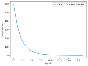
Let’s see how the loss for both techniques diminishes during model training now that we have trained our model using batch gradient descent and stochastic gradient descent. Consequently, this is how the batch gradient descent graph appears.
...
plt.plot(loss_BGD, label="Batch Gradient Descent")
plt.xlabel('Epoch')
plt.ylabel('Cost/Total loss')
plt.legend()
plt.show()

The loss history of batch gradient descent
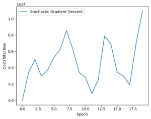
Similar to that, here is how the stochastic gradient descent graph appears.
plt.plot(loss_SGD,label="Stochastic Gradient Descent")
plt.xlabel('Epoch')
plt.ylabel('Cost/Total loss')
plt.legend()
plt.show()

Loss history of stochastic gradient descent
As you can see, the loss for batch gradient descent reduces steadily. For stochastic gradient descent, on the other hand, you’ll notice variations in the graph. The cause is pretty straightforward, as was before indicated. In batch gradient descent, the loss is updated following the processing of all training samples, whereas stochastic gradient descent updates the loss following the processing of each training sample in the training set.
After putting everything together, the following is the full code:
import torch
import numpy as np
import matplotlib.pyplot as plt

# Creating a function f(X) with a slope of -5
X = torch.arange(-5, 5, 0.1).view(-1, 1)
func = -5 * X

# Adding Gaussian noise to the function f(X) and saving it in Y
Y = func + 0.4 * torch.randn(X.size())

# Plot and visualizing the data points in blue
plt.plot(X.numpy(), Y.numpy(), 'b+', label='Y')
plt.plot(X.numpy(), func.numpy(), 'r', label='func')
plt.xlabel('x')
plt.ylabel('y')
plt.legend()
plt.grid('True', color='y')
plt.show()

# defining the function for forward pass for prediction
def forward(x):
return w * x + b

# evaluating data points with Mean Square Error (MSE)
def criterion(y_pred, y):
return torch.mean((y_pred - y) ** 2)

# Batch gradient descent
w = torch.tensor(-10.0, requires_grad=True)
b = torch.tensor(-20.0, requires_grad=True)
step_size = 0.1
loss_BGD = []
n_iter = 20

for i in range (n_iter):
# making predictions with forward pass
Y_pred = forward(X)
# calculating the loss between original and predicted data points
loss = criterion(Y_pred, Y)
# storing the calculated loss in a list
loss_BGD.append(loss.item())
# backward pass for computing the gradients of the loss w.r.t to learnable parameters
loss.backward()
# updateing the parameters after each iteration
w.data = w.data - step_size * w.grad.data
b.data = b.data - step_size * b.grad.data
# zeroing gradients after each iteration
w.grad.data.zero_()
b.grad.data.zero_()
# priting the values for understanding
print('{}, \t{}, \t{}, \t{}'.format(i, loss.item(), w.item(), b.item()))

# Stochastic gradient descent
w = torch.tensor(-10.0, requires_grad=True)
b = torch.tensor(-20.0, requires_grad=True)
step_size = 0.1
loss_SGD = []
n_iter = 20

for i in range(n_iter):
# calculating true loss and storing it
Y_pred = forward(X)
# store the loss in the list
loss_SGD.append(criterion(Y_pred, Y).tolist())

for x, y in zip(X, Y):
# making a pridiction in forward pass
y_hat = forward(x)
# calculating the loss between original and predicted data points
loss = criterion(y_hat, y)
# backward pass for computing the gradients of the loss w.r.t to learnable parameters
loss.backward()
# updateing the parameters after each iteration
w.data = w.data - step_size * w.grad.data
b.data = b.data - step_size * b.grad.data
# zeroing gradients after each iteration
w.grad.data.zero_()
b.grad.data.zero_()
# priting the values for understanding
print('{}, \t{}, \t{}, \t{}'.format(i, loss.item(), w.item(), b.item()))

# Plot graphs
plt.plot(loss_BGD, label="Batch Gradient Descent")
plt.xlabel('Epoch')
plt.ylabel('Cost/Total loss')
plt.legend()
plt.show()

plt.plot(loss_SGD,label="Stochastic Gradient Descent")
plt.xlabel('Epoch')
plt.ylabel('Cost/Total loss')
plt.legend()
plt.show()
Summary
You learned about the Gradient Descent in this tutorial, as well as several of its variations and how to use them in PyTorch. You learned specifically about:
- The Gradient Descent technique and PyTorch’s implementation
- Batch Gradient Descent and PyTorch’s use of it
- Stochastic Gradient Descent and PyTorch’s use of it
- What distinguishes Stochastic Gradient Descent from Batch Gradient Descent
- How loss diminishes during training in batch gradient descent versus stochastic gradient descent
Source link


