Fundamentals of ML with Scikit-Learn & TensorFlow

Why Use Machine Learning?

Machine Learning is the science (and art) of programming computers so they can learn from data

Here is a slightly more general definition:

[Machine Learning is the] field of study that gives computers the ability to learn without being explicitly programmed.

—Arthur Samuel, 1959

And a more engineering-oriented one:

A computer program is said to learn from experience E with respect to some task T and some performance measure P, if its performance on T, as measured by P, improves with experience E.

—Tom Mitchell, 1997

For example, your spam filter is a Machine Learning program that can learn to flag spam given examples of spam emails (e.g., flagged by users) and examples of regular (nonspam, also called “ham”) emails. The examples that the system uses to learn are called the training set. Each training example is called a training instance (or sample). In this case, the task T is to flag spam for new emails, the experience E is the training data, and the performance measure P needs to be defined; for example, you can use the ratio of correctly classified emails. This particular performance measure is called accuracy and it is often used in classification tasks.

If you just download a copy of Wikipedia, your computer has a lot more data, but it is not suddenly better at any task. Thus, it is not Machine Learning.

Why Use Machine Learning?

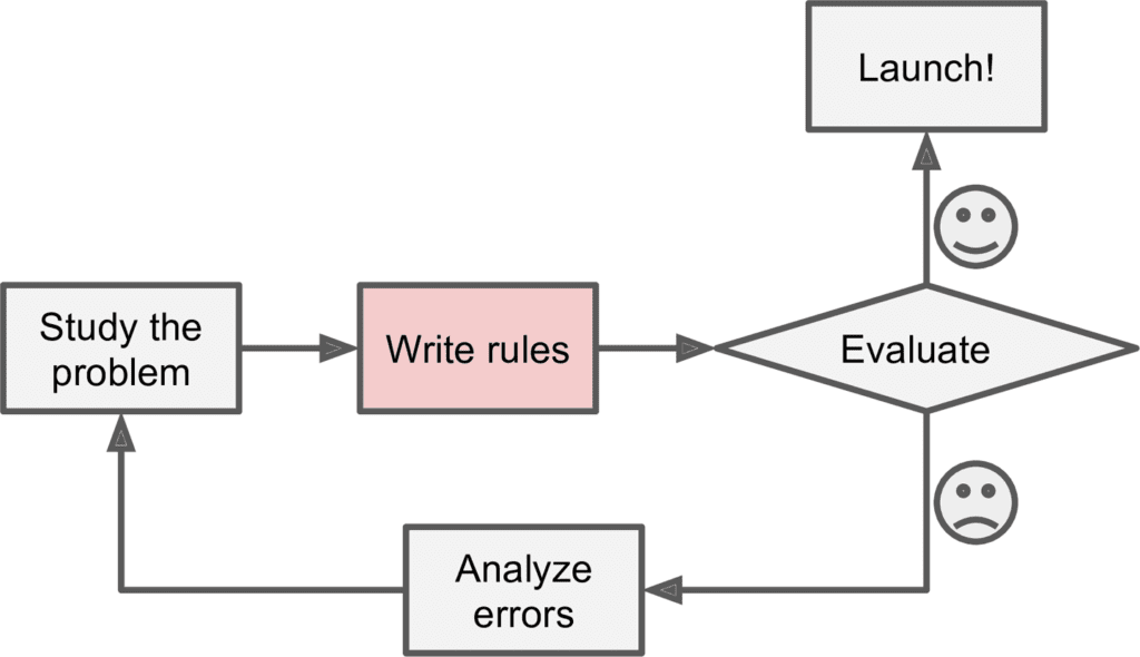
Consider how you would write a spam filter using traditional programming techni‐ ques (Figure 1-1):

1. First you would look at what spam typically looks like. You might notice that some words or phrases (such as “4U,” “credit card,” “free,” and “amazing”) tend to come up a lot in the subject. Perhaps you would also notice a few other patterns in the sender’s name, the email’s body, and so on.

2. You would write a detection algorithm for each of the patterns that you noticed, and your program would flag emails as spam if a number of these patterns are detected.

3. You would test your program, and repeat steps 1 and 2 until it is good enough.

Since the problem is not trivial, your program will likely become a long list of com‐ plex rules—pretty hard to maintain.

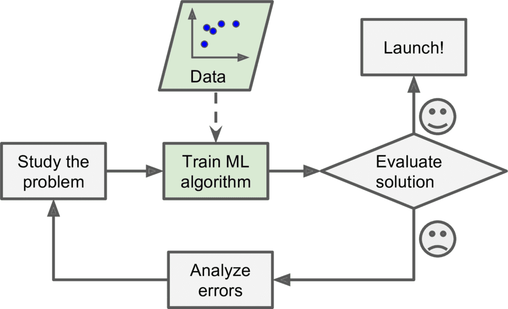
In contrast, a spam filter based on Machine Learning techniques automatically learns which words and phrases are good predictors of spam by detecting unusually fre‐ quent patterns of words in the spam examples compared to the ham examples (Figure 1-2). The program is much shorter, easier to maintain, and most likely more accurate.

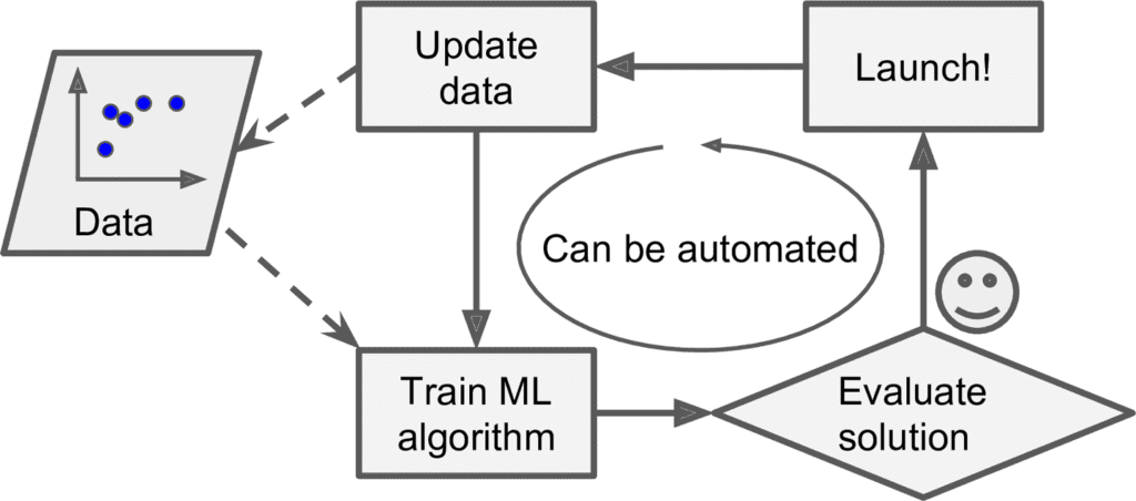
Moreover, if spammers notice that all their emails containing “4U” are blocked, they might start writing “For U” instead. A spam filter using traditional programming techniques would need to be updated to flag “For U” emails. If spammers keep working around your spam filter, you will need to keep writing new rules forever. In contrast, a spam filter based on Machine Learning techniques automatically notices that “For U” has become unusually frequent in spam flagged by users, and it starts flagging them without your intervention (Figure 1-3).

Another area where Machine Learning shines is for problems that either are too complex for traditional approaches or have no known algorithm. For example, consider speech recognition: say you want to start simple and write a program capable of distinguishing the words “one” and “two.” You might notice that the word “two” starts with a high-pitch sound (“T”), so you could hardcode an algorithm that measures high-pitch sound intensity and use that to distinguish ones and twos. Obviously this technique will not scale to thousands of words spoken by millions of very different people in noisy environments and in dozens of languages. The best solution (at least today) is to write an algorithm that learns by itself, given many example recordings for each word.

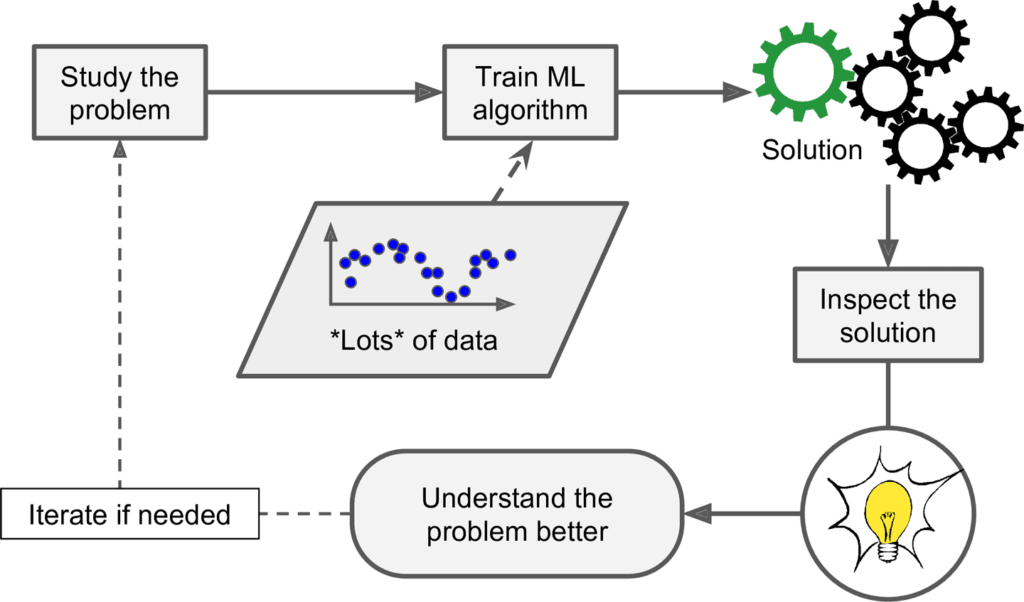
Finally, Machine Learning can help humans learn (Figure 1-4): ML algorithms can be inspected to see what they have learned (although for some algorithms this can be tricky). For instance, once the spam filter has been trained on enough spam, it can easily be inspected to reveal the list of words and combinations of words that it believes are the best predictors of spam. Sometimes this will reveal unsuspected cor‐ relations or new trends, and thereby lead to a better understanding of the problem.

Applying ML techniques to dig into large amounts of data can help discover patterns that were not immediately apparent. This is called data mining.

To summarize, Machine Learning is great for:

• Problems for which existing solutions require a lot of hand-tuning or long lists of rules: one Machine Learning algorithm can often simplify code and perform better.

• Complex problems for which there is no good solution at all using a traditional approach: the best Machine Learning techniques can find a solution.

• Fluctuating environments: a Machine Learning system can adapt to new data.

• Getting insights about complex problems and large amounts of data.

Types of Machine Learning Systems

There are so many different types of Machine Learning systems that it is useful to classify them in broad categories based on:

• Whether or not they are trained with human supervision (supervised, unsupervised, semisupervised, and Reinforcement Learning)

• Whether or not they can learn incrementally on the fly (online versus batch learning)

• Whether they work by simply comparing new data points to known data points, or instead detect patterns in the training data and build a predictive model, much like scientists do (instance-based versus model-based learning)

These criteria are not exclusive; you can combine them in any way you like. For example, a state-of-the-art spam filter may learn on the fly using a deep neural network model trained using examples of spam and ham; this makes it an online, modelbased, supervised learning system.

Let’s look at each of these criteria a bit more closely.

Supervised/Unsupervised Learning

Machine Learning systems can be classified according to the amount and type of supervision they get during training. There are four major categories: supervised learning, unsupervised learning, semisupervised learning, and Reinforcement Learning.

Supervised learning

In supervised learning, the training data you feed to the algorithm includes the desired solutions, called labels (Figure 1-5).

A typical supervised learning task is classification. The spam filter is a good example of this: it is trained with many example emails along with their class (spam or ham), and it must learn how to classify new emails.

Another typical task is to predict a target numeric value, such as the price of a car, given a set of features (mileage, age, brand, etc.) called predictors. This sort of task is called regression (Figure 1-6).1 To train the system, you need to give it many examples of cars, including both their predictors and their labels (i.e., their prices).

In Machine Learning an attribute is a data type (e.g., “Mileage”), while a feature has several meanings depending on the context, but generally means an attribute plus its value (e.g., “Mileage = 15,000”). Many people use the words attribute and feature inter‐ changeably, though.

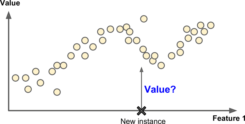
Note that some regression algorithms can be used for classification as well, and vice versa. For example, Logistic Regression is commonly used for classification, as it can output a value that corresponds to the probability of belonging to a given class (e.g., 20% chance of being spam).

Here are some of the most important supervised learning algorithms (covered in this book):

• k-Nearest Neighbors
• Linear Regression
• Logistic Regression
• Support Vector Machines (SVMs)
• Decision Trees and Random Forests
• Neural networks

Unsupervised learning

In unsupervised learning, as you might guess, the training data is unlabeled (Figure 1-7). The system tries to learn without a teacher.

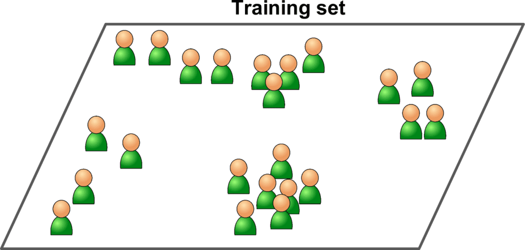
Here are some of the most important unsupervised learning algorithms

• Clustering

• Principal Component Analysis (PCA)
• Kernel PCA
• Locally-Linear Embedding (LLE)
• t-distributed Stochastic Neighbor Embedding (t-SNE)

• Association rule learning

• Apriori
• Eclat

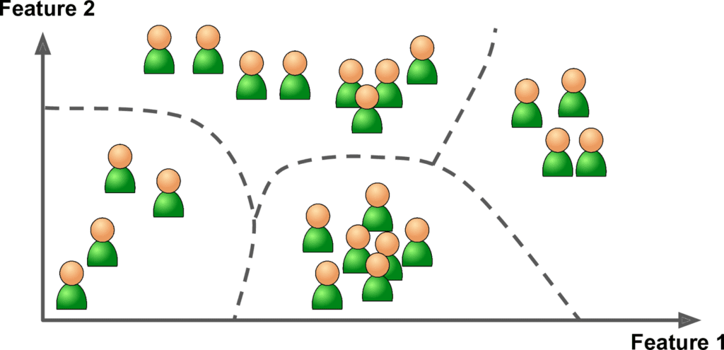
For example, say you have a lot of data about your blog’s visitors. You may want to run a clustering algorithm to try to detect groups of similar visitors (Figure 1-8). At no point do you tell the algorithm which group a visitor belongs to: it finds those connections without your help. For example, it might notice that 40% of your visitors are males who love comic books and generally read your blog in the evening, while 20% are young sci-fi lovers who visit during the weekends, and so on. If you use a hierarchical clustering algorithm, it may also subdivide each group into smaller groups. This may help you target your posts for each group.

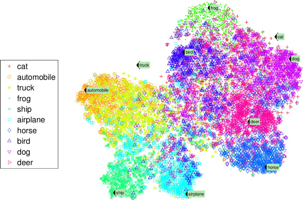
Visualization algorithms are also good examples of unsupervised learning algorithms: you feed them a lot of complex and unlabeled data, and they output a 2D or 3D representation of your data that can easily be plotted (Figure 1-9). These algorithms try to preserve as much structure as they can (e.g., trying to keep separate clusters in the input space from overlapping in the visualization), so you can understand how the data is organized and perhaps identify unsuspected patterns.

A related task is dimensionality reduction, in which the goal is to simplify the data without losing too much information. One way to do this is to merge several correlated features into one. For example, a car’s mileage may be very correlated with its age, so the dimensionality reduction algorithm will merge them into one feature that rep‐ resents the car’s wear and tear. This is called feature extraction.

It is often a good idea to try to reduce the dimension of your train‐ ing data using a dimensionality reduction algorithm before you feed it to another Machine Learning algorithm (such as a super‐ vised learning algorithm). It will run much faster, the data will take up less disk and memory space, and in some cases it may also per‐ form better.

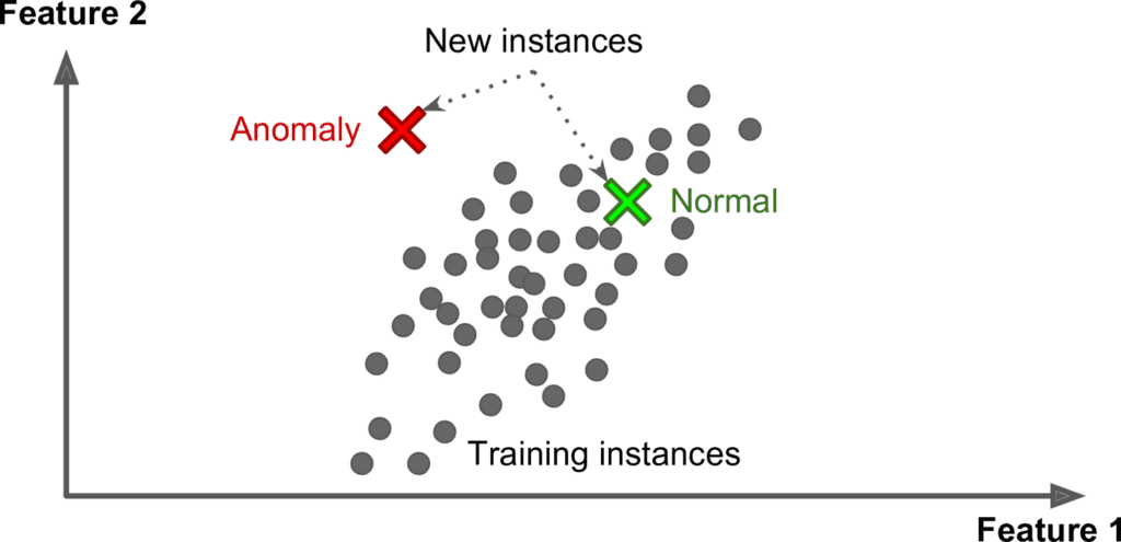
Yet another important unsupervised task is anomaly detection—for example, detect‐ ing unusual credit card transactions to prevent fraud, catching manufacturing defects, or automatically removing outliers from a dataset before feeding it to another learn‐ ing algorithm. The system is trained with normal instances, and when it sees a new instance it can tell whether it looks like a normal one or whether it is likely an anomaly (see Figure 1-10).

Finally, another common unsupervised task is association rule learning, in which the goal is to dig into large amounts of data and discover interesting relations between attributes. For example, suppose you own a supermarket. Running an association rule on your sales logs may reveal that people who purchase barbecue sauce and potato chips also tend to buy steak. Thus, you may want to place these items close to each other.

Semisupervised learning

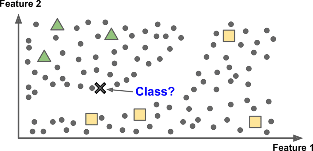
Some algorithms can deal with partially labeled training data, usually a lot of unla‐ beled data and a little bit of labeled data. This is called semisupervised learning (Figure 1-11).

Some photo-hosting services, such as Google Photos, are good examples of this. Once you upload all your family photos to the service, it automatically recognizes that the same person A shows up in photos 1, 5, and 11, while another person B shows up in photos 2, 5, and 7. This is the unsupervised part of the algorithm (clustering). Now all the system needs is for you to tell it who these people are. Just one label per person,4 and it is able to name everyone in every photo, which is useful for searching photos.

Most semisupervised learning algorithms are combinations of unsupervised and supervised algorithms. For example, deep belief networks (DBNs) are based on unsu‐ pervised components called restricted Boltzmann machines (RBMs) stacked on top of one another. RBMs are trained sequentially in an unsupervised manner, and then the whole system is fine-tuned using supervised learning techniques.

Reinforcement Learning

Reinforcement Learning is a very different beast. The learning system, called an agent in this context, can observe the environment, select and perform actions, and get rewards in return (or penalties in the form of negative rewards, as in Figure 1-12). It must then learn by itself what is the best strategy, called a policy, to get the most reward over time. A policy defines what action the agent should choose when it is in a given situation.

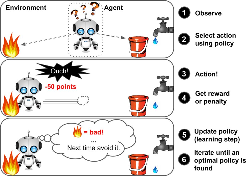
For example, many robots implement Reinforcement Learning algorithms to learn how to walk. DeepMind’s AlphaGo program is also a good example of Reinforcement Learning: it made the headlines in March 2016 when it beat the world champion Lee Sedol at the game of Go. It learned its winning policy by analyzing millions of games, and then playing many games against itself. Note that learning was turned off during the games against the champion; AlphaGo was just applying the policy it had learned.

Batch and Online Learning

Another criterion used to classify Machine Learning systems is whether or not the system can learn incrementally from a stream of incoming data.

Batch learning

In batch learning, the system is incapable of learning incrementally: it must be trained using all the available data. This will generally take a lot of time and computing resources, so it is typically done offline. First the system is trained, and then it is launched into production and runs without learning anymore; it just applies what it has learned. This is called offline learning.

If you want a batch learning system to know about new data (such as a new type of spam), you need to train a new version of the system from scratch on the full dataset (not just the new data, but also the old data), then stop the old system and replace it with the new one.

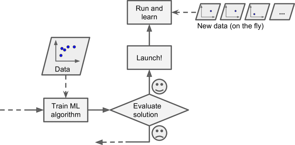
Fortunately, the whole process of training, evaluating, and launching a Machine Learning system can be automated fairly easily (as shown in Figure 1-3), so even a batch learning system can adapt to change. Simply update the data and train a new version of the system from scratch as often as needed.

This solution is simple and often works fine, but training using the full set of data can take many hours, so you would typically train a new system only every 24 hours or even just weekly. If your system needs to adapt to rapidly changing data (e.g., to pre‐ dict stock prices), then you need a more reactive solution.

Also, training on the full set of data requires a lot of computing resources (CPU, memory space, disk space, disk I/O, network I/O, etc.). If you have a lot of data and you automate your system to train from scratch every day, it will end up costing you a lot of money. If the amount of data is huge, it may even be impossible to use a batch learning algorithm.

Finally, if your system needs to be able to learn autonomously and it has limited resources (e.g., a smartphone application or a rover on Mars), then carrying around large amounts of training data and taking up a lot of resources to train for hours every day is a showstopper.

Fortunately, a better option in all these cases is to use algorithms that are capable of learning incrementally.

Online learning

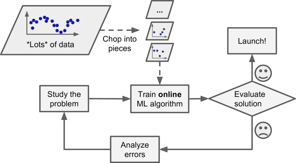
In online learning, you train the system incrementally by feeding it data instances sequentially, either individually or by small groups called mini-batches. Each learning step is fast and cheap, so the system can learn about new data on the fly, as it arrives (see Figure 1-13).

Online learning is great for systems that receive data as a continuous flow (e.g., stock prices) and need to adapt to change rapidly or autonomously. It is also a good option if you have limited computing resources: once an online learning system has learned about new data instances, it does not need them anymore, so you can discard them (unless you want to be able to roll back to a previous state and “replay” the data). This can save a huge amount of space.

Online learning algorithms can also be used to train systems on huge datasets that cannot fit in one machine’s main memory (this is called out-of-core learning). The algorithm loads part of the data, runs a training step on that data, and repeats the process until it has run on all of the data (see Figure 1-14).

This whole process is usually done offline (i.e., not on the live sys‐ tem), so online learning can be a confusing name. Think of it as incremental learning

One important parameter of online learning systems is how fast they should adapt to changing data: this is called the learning rate. If you set a high learning rate, then your system will rapidly adapt to new data, but it will also tend to quickly forget the old data (you don’t want a spam filter to flag only the latest kinds of spam it was shown). Conversely, if you set a low learning rate, the system will have more inertia; that is, it will learn more slowly, but it will also be less sensitive to noise in the new data or to sequences of nonrepresentative data points.

A big challenge with online learning is that if bad data is fed to the system, the sys‐ tem’s performance will gradually decline. If we are talking about a live system, your clients will notice. For example, bad data could come from a malfunctioning sensor on a robot, or from someone spamming a search engine to try to rank high in search results. To reduce this risk, you need to monitor your system closely and promptly switch learning off (and possibly revert to a previously working state) if you detect a drop in performance. You may also want to monitor the input data and react to abnormal data (e.g., using an anomaly detection algorithm).

Instance-Based Versus Model-Based Learning

One more way to categorize Machine Learning systems is by how they generalize. Most Machine Learning tasks are about making predictions. This means that given a number of training examples, the system needs to be able to generalize to examples it has never seen before. Having a good performance measure on the training data is good, but insufficient; the true goal is to perform well on new instances.

There are two main approaches to generalization: instance-based learning and model-based learning.

Instance-based learning

Possibly the most trivial form of learning is simply to learn by heart. If you were to create a spam filter this way, it would just flag all emails that are identical to emails that have already been flagged by users—not the worst solution, but certainly not the best.

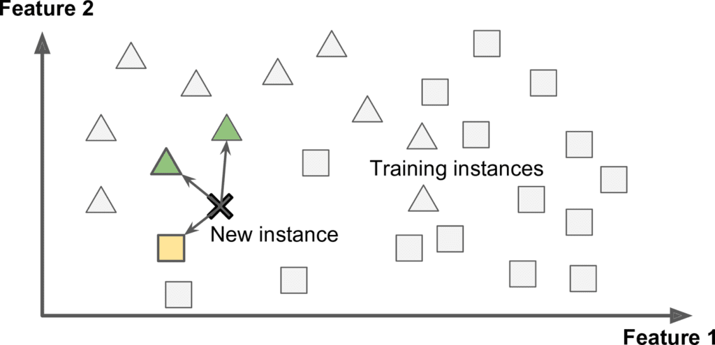
Instead of just flagging emails that are identical to known spam emails, your spam filter could be programmed to also flag emails that are very similar to known spam emails. This requires a measure of similarity between two emails. A (very basic) simi‐ larity measure between two emails could be to count the number of words they have in common. The system would flag an email as spam if it has many words in com‐ mon with a known spam email.

This is called instance-based learning: the system learns the examples by heart, then generalizes to new cases using a similarity measure (Figure 1-15).

Model-based learning

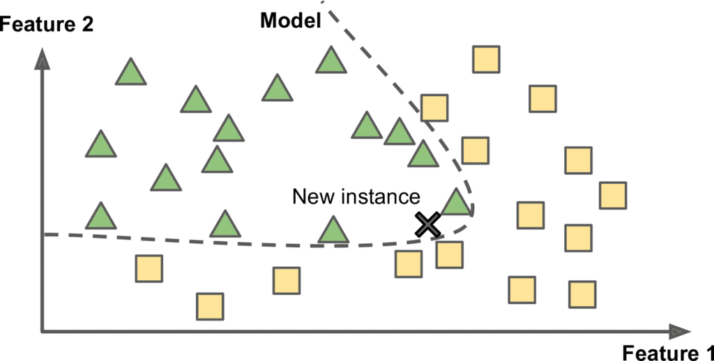
Another way to generalize from a set of examples is to build a model of these exam‐ ples, then use that model to make predictions. This is called model-based learning (Figure 1-16).

For example, suppose you want to know if money makes people happy, so you down‐ load the Better Life Index data from the OECD’s website as well as stats about GDP per capita from the IMF’s website. Then you join the tables and sort by GDP per cap‐ ita. Table 1-1 shows an excerpt of what you get.

Country	GDP per capita (USD)	Life satisfaction
Hungary	12,240	4.9
Korea	27,195	5.8
France	37,675	6.5
Australia	50,962	7.3
United States	55,805	7.2

Let’s plot the data for a few random countries (Figure 1-17).

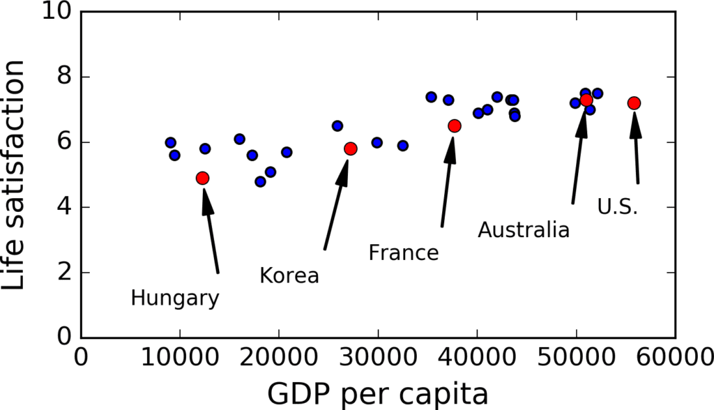
There does seem to be a trend here! Although the data is noisy (i.e., partly random), it looks like life satisfaction goes up more or less linearly as the country’s GDP per cap‐ ita increases. So you decide to model life satisfaction as a linear function of GDP per capita. This step is called model selection: you selected a linear model of life satisfac‐ tion with just one attribute, GDP per capita (Equation 1-1).

Equation 1-1. A simple linear model

li f e_satis f action = θ0 + θ1 × GDP_per_capita

This model has two model parameters, θ0 and θ1 . 5 By tweaking these parameters, you can make your model represent any linear function, as shown in Figure 1-18.

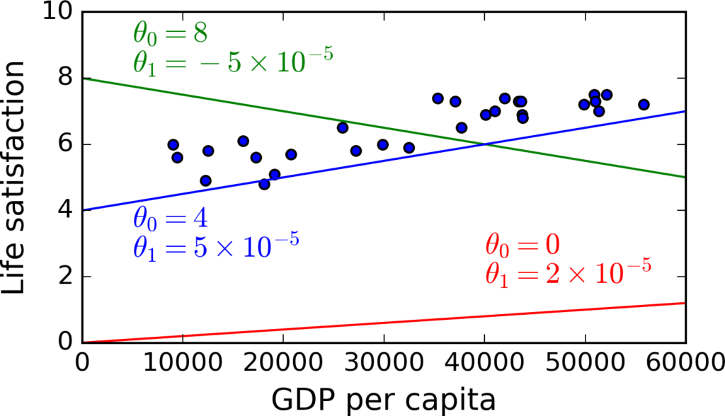
Before you can use your model, you need to define the parameter values θ0 and θ1 . How can you know which values will make your model perform best? To answer this question, you need to specify a performance measure. You can either define a utility function (or fitness function) that measures how good your model is, or you can define a cost function that measures how bad it is. For linear regression problems, people typically use a cost function that measures the distance between the linear model’s predictions and the training examples; the objective is to minimize this distance.

This is where the Linear Regression algorithm comes in: you feed it your training examples and it finds the parameters that make the linear model fit best to your data. This is called training the model. In our case the algorithm finds that the optimal parameter values are θ0 = 4.85 and θ1 = 4.91 × 10^(–5) .

Now the model fits the training data as closely as possible (for a linear model), as you can see in Figure 1-19.

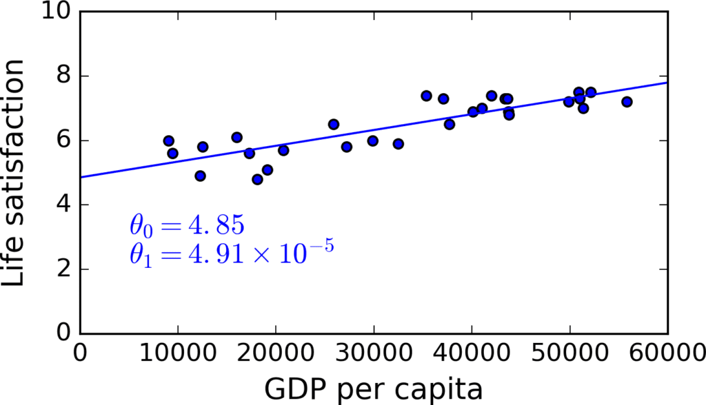
You are finally ready to run the model to make predictions. For example, say you want to know how happy Cypriots are, and the OECD data does not have the answer. Fortunately, you can use your model to make a good prediction: you look up Cyprus’s GDP per capita, find $22,587, and then apply your model and find that life satisfac‐ tion is likely to be somewhere around 4.85 + 22,587 × 4.91 × 10^(-5) = 5.96.

To whet your appetite, Example 1-1 shows the Python code that loads the data, pre‐ pares it,6 creates a scatterplot for visualization, and then trains a linear model and makes a prediction.

Example 1-1. Training and running a linear model using Scikit-Learn

import matplotlib
import matplotlib.pyplot as plt
import numpy as np
import pandas as pd
import sklearn

# Load the data
oecd_bli = pd.read_csv("oecd_bli_2015.csv", thousands=',')
gdp_per_capita = pd.read_csv("gdp_per_capita.csv",thousands=',',delimiter='\t',
 encoding='latin1', na_values="n/a")

# Prepare the data
country_stats = prepare_country_stats(oecd_bli, gdp_per_capita)
X = np.c_[country_stats["GDP per capita"]]
y = np.c_[country_stats["Life satisfaction"]]

# Visualize the data
country_stats.plot(kind='scatter', x="GDP per capita", y='Life satisfaction')
plt.show()

# Select a linear model
lin_reg_model = sklearn.linear_model.LinearRegression()

# Train the model
lin_reg_model.fit(X, y)

# Make a prediction for Cyprus
X_new = [[22587]] # Cyprus' GDP per capita
print(lin_reg_model.predict(X_new)) # outputs [[ 5.96242338]]

If you had used an instance-based learning algorithm instead, you would have found that Slovenia has the closest GDP per capita to that of Cyprus ($20,732), and since the OECD data tells us that Slovenians’ life satisfaction is 5.7, you would have predicted a life satisfaction of 5.7 for Cyprus. If you zoom out a bit and look at the two next closest countries, you will find Portugal and Spain with life satisfactions of 5.1 and 6.5, respectively. Averaging these three values, you get 5.77, which is pretty close to your model-based pre‐ diction. This simple algorithm is called k-Nearest Neighbors regres‐ sion (in this example, k = 3).

Replacing the Linear Regression model with k-Nearest Neighbors regression in the previous code is as simple as replacing this line:

clf = sklearn.linear_model.LinearRegression()

with this one:

clf = sklearn.neighbors.KNeighborsRegressor(n_neighbors=3)

If all went well, your model will make good predictions. If not, you may need to use more attributes (employment rate, health, air pollution, etc.), get more or better qual‐ ity training data, or perhaps select a more powerful model (e.g., a Polynomial Regres‐ sion model).

• You studied the data
• You selected a model.
• You trained it on the training data (i.e., the learning algorithm searched for the model parameter values that minimize a cost function).
• Finally, you applied the model to make predictions on new cases (this is called inference), hoping that this model will generalize well.

We have covered a lot of ground so far: you now know what Machine Learning is really about, why it is useful, what some of the most common categories of ML sys‐ tems are, and what a typical project workflow looks like. Now let’s look at what can go wrong in learning and prevent you from making accurate predictions.

Main Challenges of Machine Learning

In short, since your main task is to select a learning algorithm and train it on some data, the two things that can go wrong are “bad algorithm” and “bad data.” Let’s start with examples of bad data.

Insuffcient Quantity of Training Data

For a toddler to learn what an apple is, all it takes is for you to point to an apple and say “apple” (possibly repeating this procedure a few times). Now the child is able to recognize apples in all sorts of colors and shapes. Genius.

Machine Learning is not quite there yet; it takes a lot of data for most Machine Learn‐ ing algorithms to work properly. Even for very simple problems you typically need thousands of examples, and for complex problems such as image or speech recogni‐ tion you may need millions of examples (unless you can reuse parts of an existing model).

---

The Unreasonable Effectiveness of Data

In a famous paper published in 2001, Microsoft researchers Michele Banko and Eric Brill showed that very different Machine Learning algorithms, including fairly simple ones, performed almost identically well on a complex problem of natural language disambiguation8 once they were given enough data (as you can see in Figure 1-20).

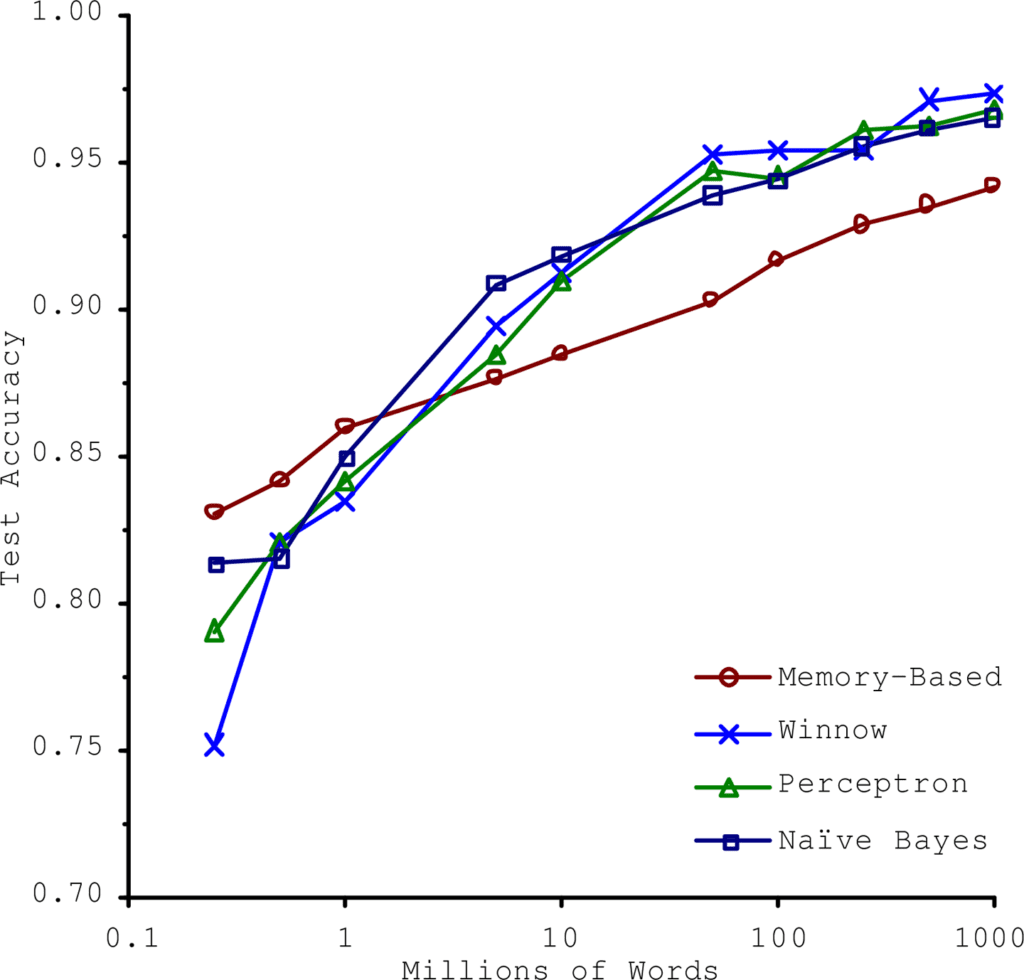
As the authors put it: “these results suggest that we may want to reconsider the tradeoff between spending time and money on algorithm development versus spending it on corpus development.”

The idea that data matters more than algorithms for complex problems was further popularized by Peter Norvig et al. in a paper titled “The Unreasonable Effectiveness of Data” published in 2009.10 It should be noted, however, that small- and mediumsized datasets are still very common, and it is not always easy or cheap to get extra training data, so don’t abandon algorithms just yet.

---

Nonrepresentative Training Data

In order to generalize well, it is crucial that your training data be representative of the new cases you want to generalize to. This is true whether you use instance-based learning or model-based learning.

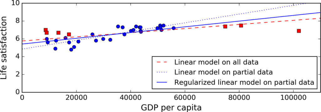
For example, the set of countries we used earlier for training the linear model was not perfectly representative; a few countries were missing. Figure 1-21 shows what the data looks like when you add the missing countries.

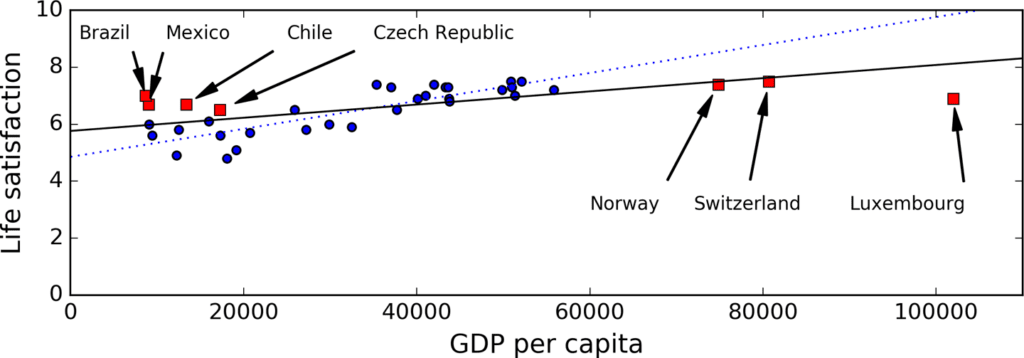
If you train a linear model on this data, you get the solid line, while the old model is represented by the dotted line. As you can see, not only does adding a few missing countries significantly alter the model, but it makes it clear that such a simple linear model is probably never going to work well. It seems that very rich countries are not happier than moderately rich countries (in fact they seem unhappier), and conversely some poor countries seem happier than many rich countries.

By using a nonrepresentative training set, we trained a model that is unlikely to make accurate predictions, especially for very poor and very rich countries.

It is crucial to use a training set that is representative of the cases you want to general‐ ize to. This is often harder than it sounds: if the sample is too small, you will have sampling noise (i.e., nonrepresentative data as a result of chance), but even very large samples can be nonrepresentative if the sampling method is flawed. This is called sampling bias.

---

A Famous Example of Sampling Bias

Perhaps the most famous example of sampling bias happened during the US presi‐ dential election in 1936, which pitted Landon against Roosevelt: the Literary Digest conducted a very large poll, sending mail to about 10 million people. It got 2.4 million answers, and predicted with high confidence that Landon would get 57% of the votes.

Instead, Roosevelt won with 62% of the votes. The flaw was in the Literary Digest’s sampling method:

• First, to obtain the addresses to send the polls to, the Literary Digest used tele‐ phone directories, lists of magazine subscribers, club membership lists, and the like. All of these lists tend to favor wealthier people, who are more likely to vote Republican (hence Landon).
• Second, less than 25% of the people who received the poll answered. Again, this introduces a sampling bias, by ruling out people who don’t care much about poli‐ tics, people who don’t like the Literary Digest, and other key groups. This is a spe‐ cial type of sampling bias called nonresponse bias.

Here is another example: say you want to build a system to recognize funk music vid‐ eos. One way to build your training set is to search “funk music” on YouTube and use the resulting videos. But this assumes that YouTube’s search engine returns a set of videos that are representative of all the funk music videos on YouTube. In reality, the search results are likely to be biased toward popular artists (and if you live in Brazil you will get a lot of “funk carioca” videos, which sound nothing like James Brown). On the other hand, how else can you get a large training set?

---

Poor-Quality Data

Obviously, if your training data is full of errors, outliers, and noise (e.g., due to poorquality measurements), it will make it harder for the system to detect the underlying patterns, so your system is less likely to perform well. It is often well worth the effort to spend time cleaning up your training data. The truth is, most data scientists spend a significant part of their time doing just that. For example:

• If some instances are clearly outliers, it may help to simply discard them or try to fix the errors manually
• If some instances are missing a few features (e.g., 5% of your customers did not specify their age), you must decide whether you want to ignore this attribute alto‐ gether, ignore these instances, fill in the missing values (e.g., with the median age), or train one model with the feature and one model without it, and so on.

Irrelevant Features

As the saying goes: garbage in, garbage out. Your system will only be capable of learn‐ ing if the training data contains enough relevant features and not too many irrelevant ones. A critical part of the success of a Machine Learning project is coming up with a good set of features to train on. This process, called feature engineering, involves:

• Feature selection: selecting the most useful features to train on among existing features.
• Feature extraction: combining existing features to produce a more useful one (as we saw earlier, dimensionality reduction algorithms can help).
• Creating new features by gathering new data.

Now that we have looked at many examples of bad data, let’s look at a couple of exam‐ ples of bad algorithms.

Overfitting the Training Data

Say you are visiting a foreign country and the taxi driver rips you off. You might be tempted to say that all taxi drivers in that country are thieves. Overgeneralizing is something that we humans do all too often, and unfortunately machines can fall into the same trap if we are not careful. In Machine Learning this is called overfitting: it means that the model performs well on the training data, but it does not generalize well.

Figure 1-22 shows an example of a high-degree polynomial life satisfaction model that strongly overfits the training data. Even though it performs much better on the training data than the simple linear model, would you really trust its predictions?

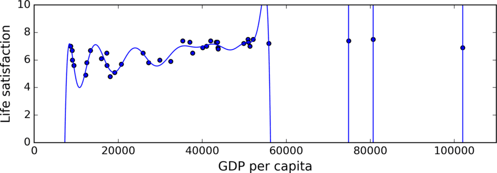
Complex models such as deep neural networks can detect subtle patterns in the data, but if the training set is noisy, or if it is too small (which introduces sampling noise), then the model is likely to detect patterns in the noise itself. Obviously these patterns will not generalize to new instances. For example, say you feed your life satisfaction model many more attributes, including uninformative ones such as the country’s name. In that case, a complex model may detect patterns like the fact that all coun‐ tries in the training data with a w in their name have a life satisfaction greater than 7: New Zealand (7.3), Norway (7.4), Sweden (7.2), and Switzerland (7.5). How confident are you that the W-satisfaction rule generalizes to Rwanda or Zimbabwe? Obviously this pattern occurred in the training data by pure chance, but the model has no way to tell whether a pattern is real or simply the result of noise in the data.

Overfitting happens when the model is too complex relative to the amount and noisiness of the training data. The possible solutions are

• To simplify the model by selecting one with fewer parameters (e.g., a linear model rather than a high-degree polynomial model), by reducing the number of attributes in the training data or by constraining the model.
• To gather more training data
• To reduce the noise in the training data (e.g., fix data errors and remove outliers)

Constraining a model to make it simpler and reduce the risk of overfitting is called regularization. For example, the linear model we defined earlier has two parameters, θ0 and θ1 . This gives the learning algorithm two degrees of freedom to adapt the model to the training data: it can tweak both the height (θ0 ) and the slope (θ1 ) of the line. If we forced θ1 = 0, the algorithm would have only one degree of freedom and would have a much harder time fitting the data properly: all it could do is move the line up or down to get as close as possible to the training instances, so it would end up around the mean. A very simple model indeed! If we allow the algorithm to modify θ1 but we force it to keep it small, then the learning algorithm will effectively have some‐ where in between one and two degrees of freedom. It will produce a simpler model than with two degrees of freedom, but more complex than with just one. You want to find the right balance between fitting the data perfectly and keeping the model simple enough to ensure that it will generalize well.

Figure 1-23 shows three models: the dotted line represents the original model that was trained with a few countries missing, the dashed line is our second model trained with all countries, and the solid line is a linear model trained with the same data as the first model but with a regularization constraint. You can see that regularization forced the model to have a smaller slope, which fits a bit less the training data that the model was trained on, but actually allows it to generalize better to new examples.

The amount of regularization to apply during learning can be controlled by a hyper‐ parameter. A hyperparameter is a parameter of a learning algorithm (not of the model). As such, it is not affected by the learning algorithm itself; it must be set prior to training and remains constant during training. If you set the regularization hyper‐ parameter to a very large value, you will get an almost flat model (a slope close to zero); the learning algorithm will almost certainly not overfit the training data, but it will be less likely to find a good solution. Tuning hyperparameters is an important part of building a Machine Learning system (you will see a detailed example in the next chapter).

Underfitting the Training Data

As you might guess, underfitting is the opposite of overfitting: it occurs when your model is too simple to learn the underlying structure of the data. For example, a lin‐ ear model of life satisfaction is prone to underfit; reality is just more complex than the model, so its predictions are bound to be inaccurate, even on the training examples.

The main options to fix this problem are:

• Selecting a more powerful model, with more parameters
• Feeding better features to the learning algorithm (feature engineering)
• Reducing the constraints on the model (e.g., reducing the regularization hyper‐ parameter)

Stepping Back

By now you already know a lot about Machine Learning. However, we went through so many concepts that you may be feeling a little lost, so let’s step back and look at the big picture:

• Machine Learning is about making machines get better at some task by learning from data, instead of having to explicitly code rules.
• There are many different types of ML systems: supervised or not, batch or online, instance-based or model-based, and so on.
• In a ML project you gather data in a training set, and you feed the training set to a learning algorithm. If the algorithm is model-based it tunes some parameters to fit the model to the training set (i.e., to make good predictions on the training set itself), and then hopefully it will be able to make good predictions on new cases as well. If the algorithm is instance-based, it just learns the examples by heart and uses a similarity measure to generalize to new instances.
• The system will not perform well if your training set is too small, or if the data is not representative, noisy, or polluted with irrelevant features (garbage in, garbage out). Lastly, your model needs to be neither too simple (in which case it will underfit) nor too complex (in which case it will overfit).

There’s just one last important topic to cover: once you have trained a model, you don’t want to just “hope” it generalizes to new cases. You want to evaluate it, and finetune it if necessary. Let’s see how.

Testing and Validating

The only way to know how well a model will generalize to new cases is to actually try it out on new cases. One way to do that is to put your model in production and moni‐ tor how well it performs. This works well, but if your model is horribly bad, your users will complain not the best idea.

A better option is to split your data into two sets: the training set and the test set. As these names imply, you train your model using the training set, and you test it using the test set. The error rate on new cases is called the generalization error (or out-ofsample error), and by evaluating your model on the test set, you get an estimation of this error. This value tells you how well your model will perform on instances it has never seen before.

If the training error is low (i.e., your model makes few mistakes on the training set) but the generalization error is high, it means that your model is overfitting the train‐ ing data.

It is common to use 80% of the data for training and hold out 20% for testing.

So evaluating a model is simple enough: just use a test set. Now suppose you are hesi‐ tating between two models (say a linear model and a polynomial model): how can you decide? One option is to train both and compare how well they generalize using the test set.

Now suppose that the linear model generalizes better, but you want to apply some regularization to avoid overfitting. The question is: how do you choose the value of the regularization hyperparameter? One option is to train 100 different models using 100 different values for this hyperparameter. Suppose you find the best hyperparame‐ ter value that produces a model with the lowest generalization error, say just 5% error.

So you launch this model into production, but unfortunately it does not perform as well as expected and produces 15% errors. What just happened?

The problem is that you measured the generalization error multiple times on the test set, and you adapted the model and hyperparameters to produce the best model for that set. This means that the model is unlikely to perform as well on new data.

A common solution to this problem is to have a second holdout set called the valida‐ tion set. You train multiple models with various hyperparameters using the training set, you select the model and hyperparameters that perform best on the validation set, and when you’re happy with your model you run a single final test against the test set to get an estimate of the generalization error.

To avoid “wasting” too much training data in validation sets, a common technique is to use cross-validation: the training set is split into complementary subsets, and each model is trained against a different combination of these subsets and validated against the remaining parts. Once the model type and hyperparameters have been selected, a final model is trained using these hyperparameters on the full training set, and the generalized error is measured on the test set.

---

No Free Lunch Theorem

A model is a simplified version of the observations. The simplifications are meant to discard the superfluous details that are unlikely to generalize to new instances. How‐ ever, to decide what data to discard and what data to keep, you must make assump‐ tions. For example, a linear model makes the assumption that the data is fundamentally linear and that the distance between the instances and the straight line is just noise, which can safely be ignored.

In a famous 1996 paper, 11 David Wolpert demonstrated that if you make absolutely no assumption about the data, then there is no reason to prefer one model over any other. This is called the No Free Lunch (NFL) theorem. For some datasets the best model is a linear model, while for other datasets it is a neural network. There is no model that is a priori guaranteed to work better (hence the name of the theorem). The only way to know for sure which model is best is to evaluate them all. Since this is not possible, in practice you make some reasonable assumptions about the data and you evaluate only a few reasonable models. For example, for simple tasks you may evalu‐ ate linear models with various levels of regularization, and for a complex problem you may evaluate various neural networks.

---

This article has been published from the source link without modifications to the text. Only the headline has been changed.

Source link