One of the most prevailing and exciting supervised learning models with associated learning algorithms that analyse data and recognise patterns is Support Vector Machines (SVMs). It is used for solving both regression and classification problems. However, it is mostly used in solving classification problems. SVMs were first introduced by B.E. Boser et al. in 1992 and has become popular due to success in handwritten digit recognition in 1994. Before the emergence of Boosting Algorithms, for example, XGBoost and AdaBoost, SVMs had been commonly used.
If you want to have a consolidated foundation of Machine Learning algorithms, you should definitely have it in your arsenal. The algorithm of SVMs is powerful, but the concepts behind are not as complicated as you think.
Problem with Logistic Regression
In my previous article, I have explained clearly what Logistic Regression is (link). It helps solve classification problems separating the instances into two classes. However, there is an infinite number of decision boundaries, and Logistic Regression only picks an arbitrary one.
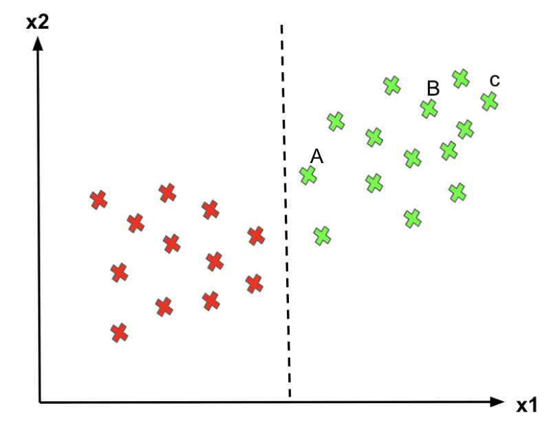
- For point C, since it’s far away from the decision boundary, we are quite certain to classify it as 1.
- For point A, even though we classify it as 1 for now, since it is pretty close to the decision boundary, if the boundary moves a little to the right, we would mark point C as “0” instead. Hence, we’re much more confident about our prediction at A than at C
Logistic Regression doesn’t care whether the instances are close to the decision boundary. Therefore, the decision boundary it picks may not be optimal. As we can see from the above graph, if a point is far from the decision boundary, we may be more confident in our predictions. Therefore, the optimal decision boundary should be able to maximize the distance between the decision boundary and all instances. i.e., maximize the margins. That’s why the SVM algorithm is important!
What is Support Vector Machines (SVMs)?
Given a set of training examples, each marked as belonging to one or the other of two categories, an SVM training algorithm builds a model that assigns new examples to one category or the other, making it a non-probabilistic binary linear classifier.
The objective of applying SVMs is to find the best line in two dimensions or the best hyperplane in more than two dimensions in order to help us separate our space into classes. The hyperplane (line) is found through the maximum margin, i.e., the maximum distance between data points of both classes.
Don’t you think the definition and idea of SVM look a bit abstract? No worries, let me explain in details.
Support Vector Machines
Imagine the labelled training set are two classes of data points (two dimensions): Alice and Cinderella. To separate the two classes, there are so many possible options of hyperplanes that separate correctly. As shown in the graph below, we can achieve exactly the same result using different hyperplanes (L1, L2, L3). However, if we add new data points, the consequence of using various hyperplanes will be very different in terms of classifying new data point into the right group of class.
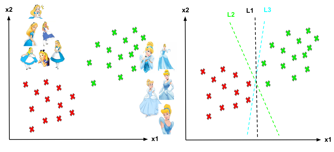
Different hyperplanes (L1, L2, L3).
How can we decide a separating line for the classes? Which hyperplane shall we use?
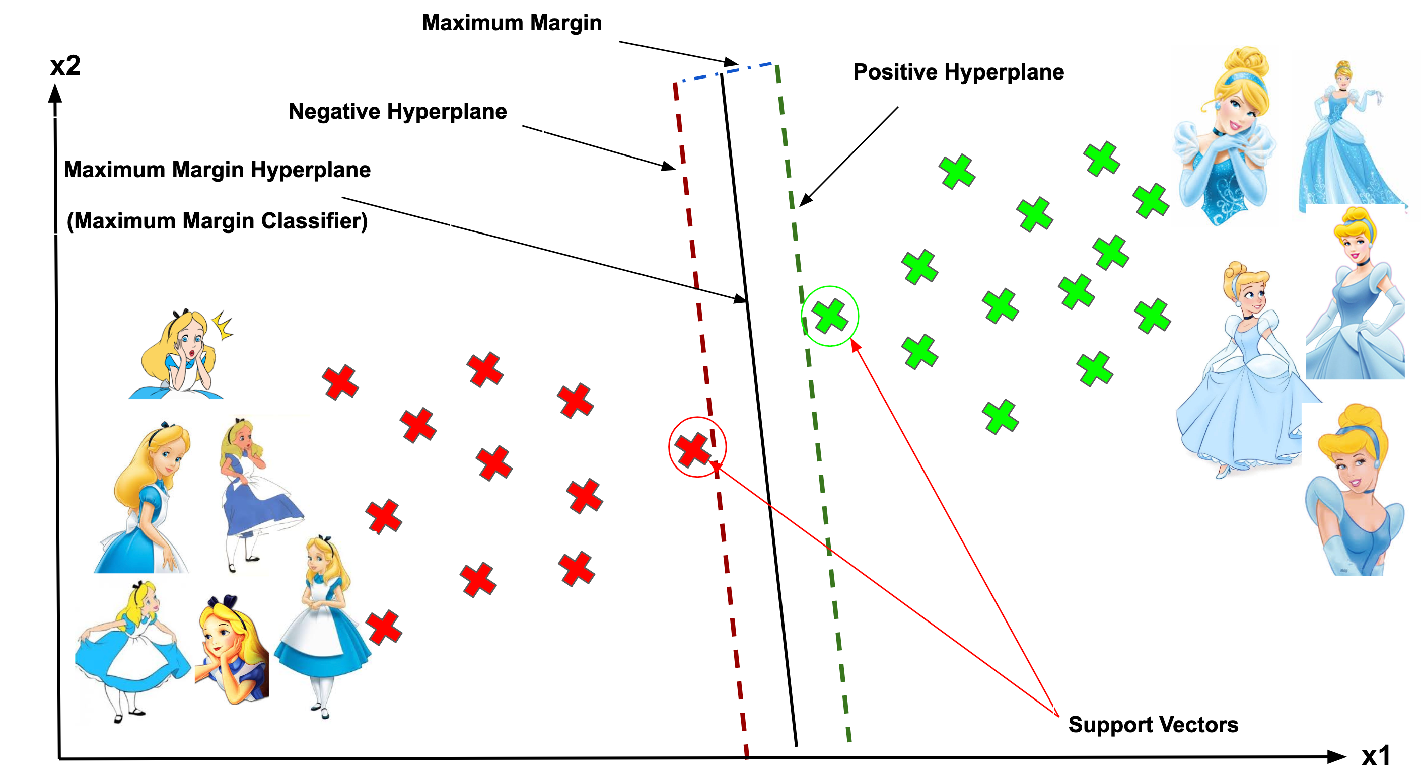
Support Vector, Hyperplane, and Margin
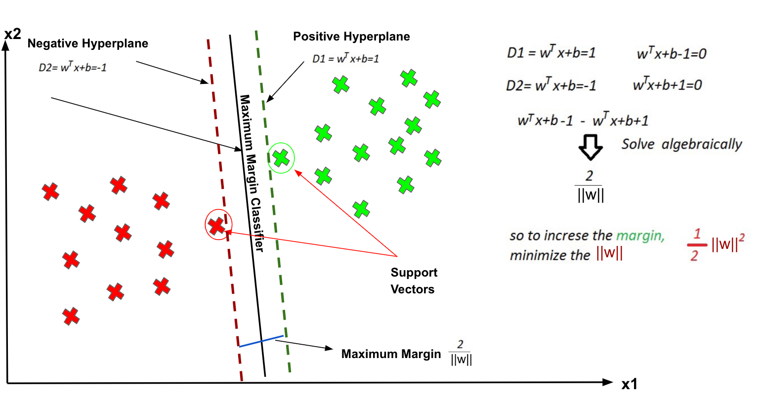
The vector points closest to the hyperplane are known as the support vector points because only these two points are contributing to the result of the algorithm, and other points are not. If a data point is not a support vector, removing it has no effect on the model. On the other hand, deleting the support vectors will then change the position of the hyperplane.
The dimension of the hyperplane depends upon the number of features. If the number of input features is 2, then the hyperplane is just a line. If the number of input features is 3, then the hyperplane becomes a two-dimensional plane. It becomes difficult to imagine when the number of features exceeds 3.
The distance of the vectors from the hyperplane is called the margin, which is a separation of a line to the closest class points. We would like to choose a hyperplane that maximises the margin between classes. The graph below shows what good margin and bad margin are.

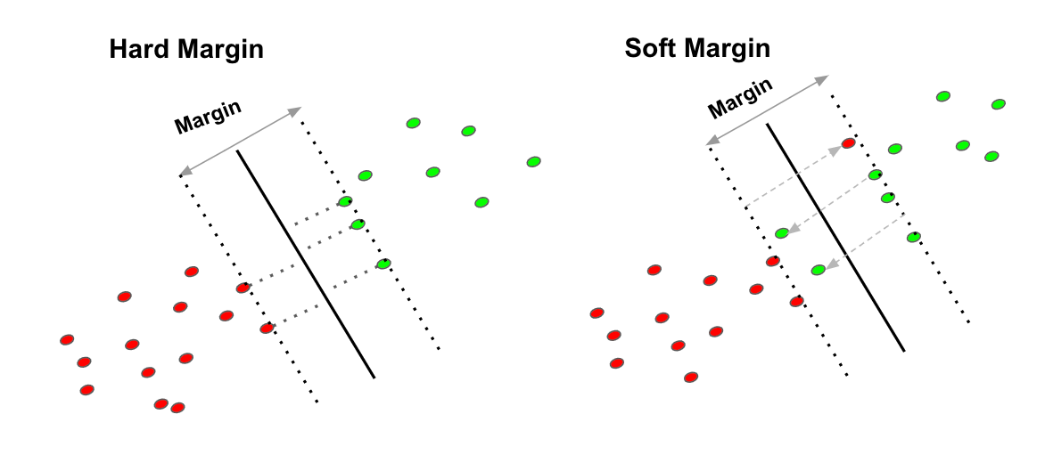
Hard Margin
If the training data is linearly separable, we can select two parallel hyperplanes that separate the two classes of data, so that the distance between them is as large as possible.
Soft Margin
As most of the real-world data are not fully linearly separable, we will allow some margin violation to occur, which is called soft margin classification. It is better to have a large margin, even though some constraints are violated. Margin violation means choosing a hyperplane, which can allow some data points to stay in either the incorrect side of the hyperplane and between the margin and the correct side of the hyperplane.
In order to find the maximal margin, we need to maximize the margin between the data points and the hyperplane. In the following session, I will share the mathematical concepts behind this algorithm.
Linear Algebra Revisited
Before we move on, let’s review some concepts in Linear Algebra.
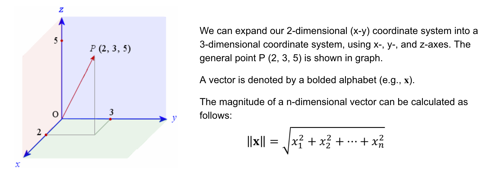

Maximising the Margin
You probably learned that an equation of a line is y=ax+b. However, you will often find that the equation of a hyperplane is defined by:
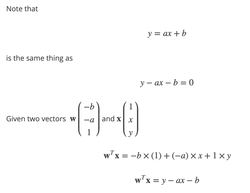
The two equations are just two different ways of expressing the same thing.
For Support Vector Classifier (SVC), we use ?T?+? where ? is the weight vector, and ? is the bias.

You can see that the name of the variables in the hyperplane equation are w and x, which means they are vectors! A vector has magnitude (size) and direction, which works perfectly well in 3 or more dimensions. Therefore, the application of “vector” is used in the SVMs algorithm.
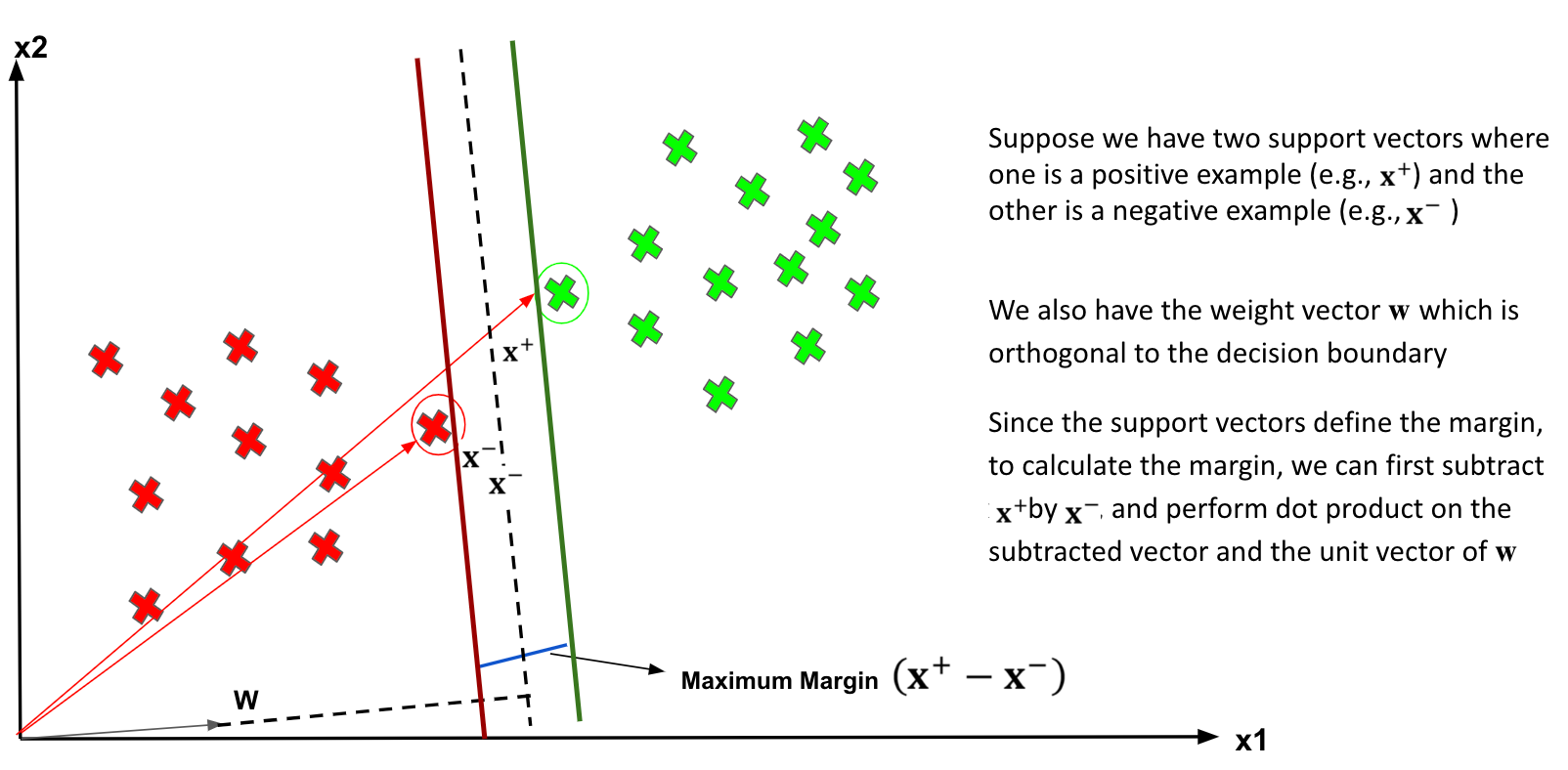

The equation of calculating the Margin.
Cost Function and Gradient Updates
Maximizing-Margin is equivalent to Minimizing Loss.
In the SVM algorithm, we are looking to maximize the margin between the data points and the hyperplane. The loss function that helps maximize the margin is hinge loss.

λ=1/C (C is always used for regularization coefficient).
The function of the first term, hinge loss, is to penalize misclassifications. It measures the error due to misclassification (or data points being closer to the classification boundary than the margin). The second term is the regularization term, which is a technique to avoid overfitting by penalizing large coefficients in the solution vector. The λ(lambda) is the regularization coefficient, and its major role is to determine the trade-off between increasing the margin size and ensuring that the xi lies on the correct side of the margin.
“Hinge” describes the fact that the error is 0 if the data point is classified correctly (and is not too close to the decision boundary).
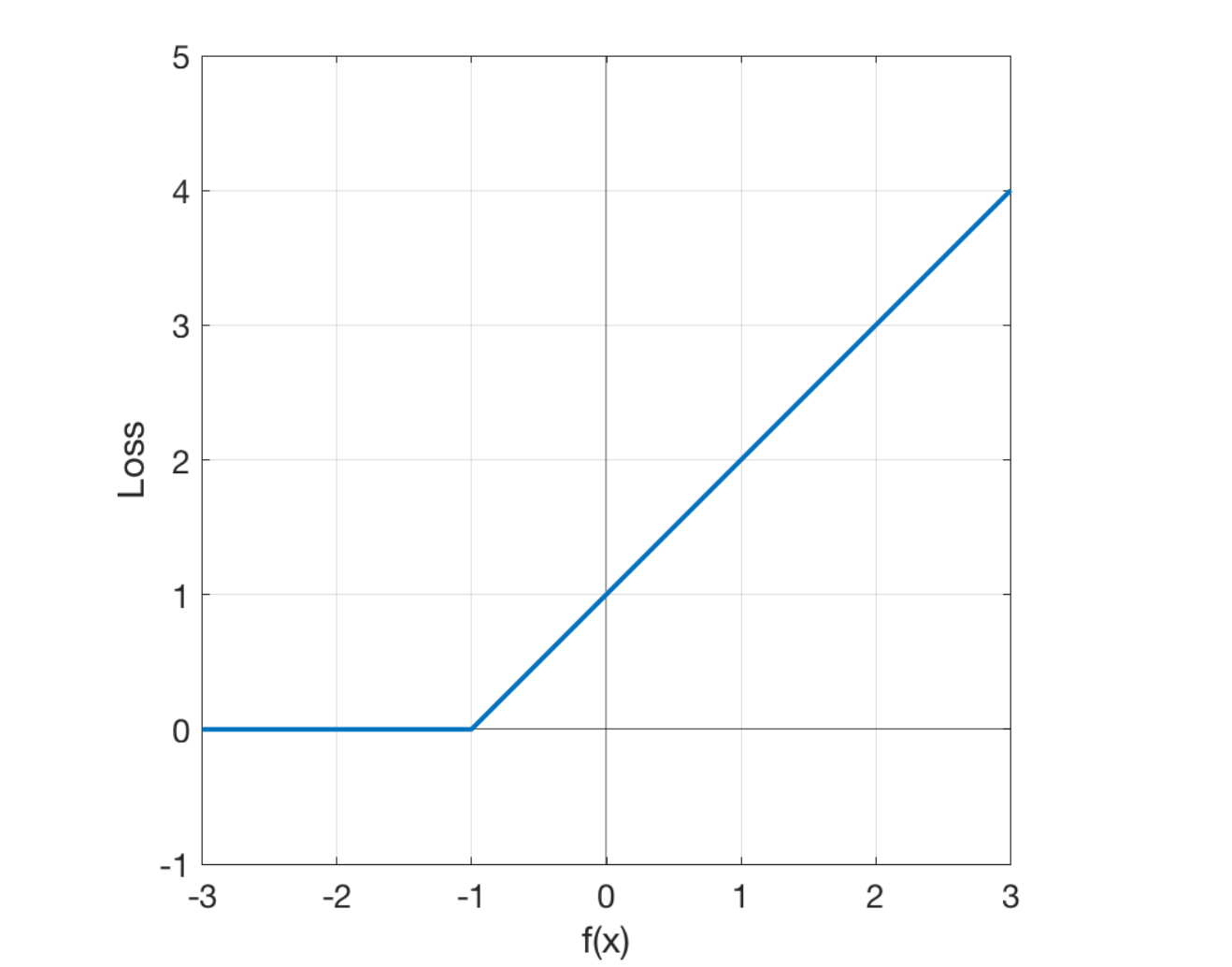
When the true class is -1 (as in your example), the hinge loss looks like this in the graph.
We need to minimise the above loss function to find the max-margin classifier.
We can derive the formula for the margin from the hinge-loss. If a data point is on the margin of the classifier, the hinge-loss is exactly zero. Hence, on the margin, we have:

Note that ?i is either +1 or -1.
Therefore, we have:

Our objective function is then:

To minimize such an objection function, we should then use Lagrange Multiplier.
Classifying non-linear data
What about data points are not linearly separable?
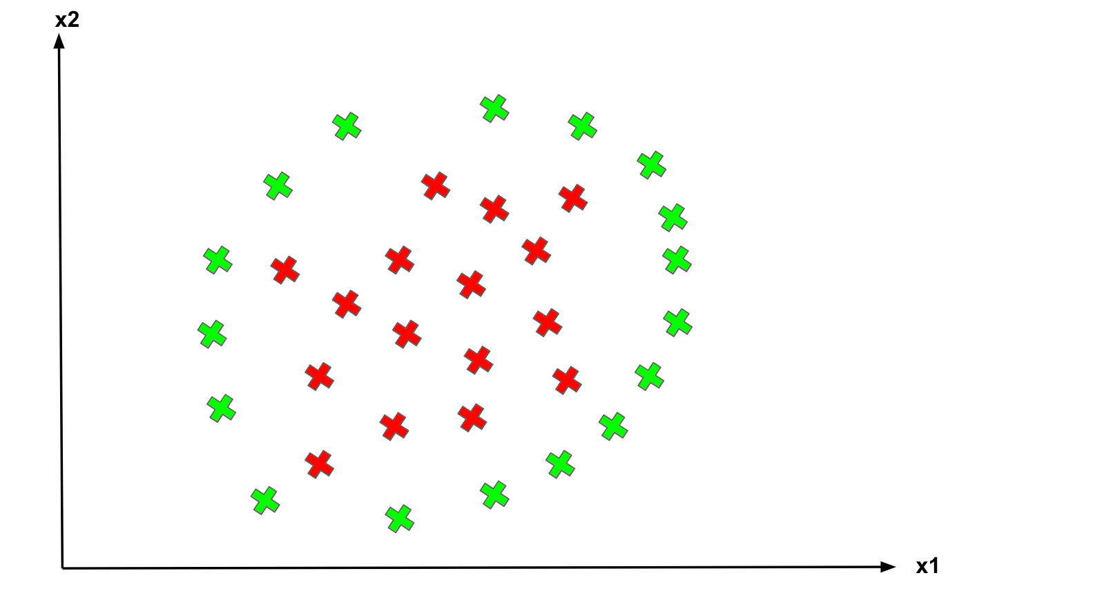
Non-linear separate.
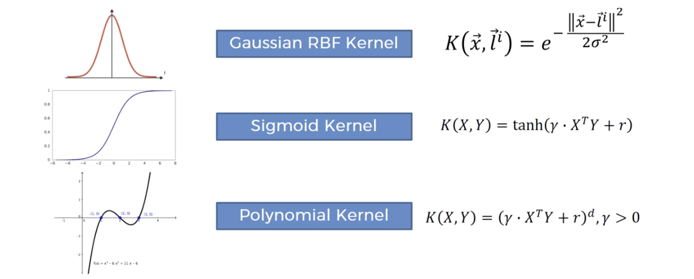
SVM has a technique called the kernel trick. These are functions that take low dimensional input space and transform it into a higher-dimensional space, i.e., it converts not separable problem to separable problem. It is mostly useful in non-linear separation problems. This is shown as follows:
Mapping to a Higher Dimension
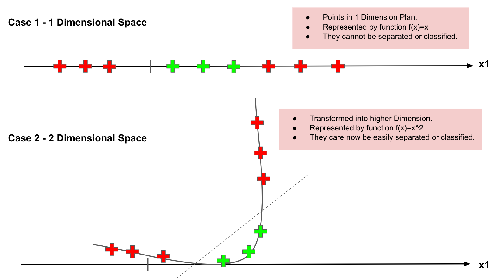
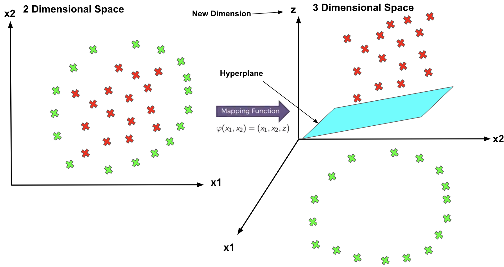
Some Frequently Used Kernels
Why SVMs
- Solve the data points are not linearly separable
- Effective in a higher dimension.
- Suitable for small data set: effective when the number of features is more than training examples.
- Overfitting problem: The hyperplane is affected by only the support vectors, so SVMs are not robust to the outliner.
Summary: Now you should know
- Problem with Logistic Regression
- What is Support Vector, Hyperplane, and Margin
- How to find the maximised margin using hinge-loss
- How to deal with non-linear separable data using different kernels
This article has been published from the source link without modifications to the text. Only the headline has been changed.
Source link


