All passionate machine learning developers enjoy a lot create, train and find out the best fitted models for their use cases. But the last remaining question is how to put these models in production and make them ready to be consumed?
In real world industry the majority of Artificial Intelligence use cases are simply limited in the POC phase, which is very frustrating 🙁 !!
In this post, we will go through the entire life-cycle of a machine learning model process: starting from data retrieving to model serving.
We will use the IBM Watson Marketing Customer Value Data gathered from Watson Analytics, to create a dash web app simulator allowing to change feature values and getting the updated score at each simulation. The app is deployed here on heroku platform. I will show you how I got that web app served, but also give you some tricks to avoid wasting a loooot of time to solve some issues that can occur while deploying a dash app.
The related github repo is here:
Step 0: I created a new repo as follows, then I cloned it:
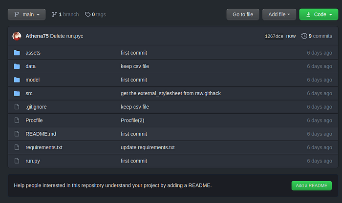
The picture above is a global structure at the the end of the project. However, you might make the same directories structures at the very beginning.
Step1 : Retrieve data:
I simply downloaded it from kaggle, you can also use the kaggle-API.
Then load the data:
import pandas as pd
df = (pd.read_csv('../data/Customer-Value-Analysis.csv')
     .set_index('Customer')
     )
Step2 : data Pre-porcessing :
In this step we can construct our own pipeline so that it can be re-used later on new incoming data.
First separate the target, numerical and categorical features:
X = df.drop(['Response'], axis = 1)
y = df.Response.apply(lambda X : 0 if X == 'No' else 1)
# categorical features
cats = [var for var, var_type in X.dtypes.items() if var_type=='object']
# numerical features
nums = [var for var in X.columns if var not in cats]
Custom Pipeline:
With many data transformation steps it is recommended to use Pipeline class provided by Scikit-learn that helps to make sequenced transformations in the right order. It can be done using the FeatureUnion estimator offered by scikit-learn. This estimator applies a list of transformer objects in parallel to the input data, then concatenates the results.
In this project, I implemented the following code (source from this kaggle notebook)
from sklearn.base import BaseEstimator, TransformerMixin
from sklearn.preprocessing import OneHotEncoder, StandardScaler
from sklearn.impute import KNNImputer
from sklearn.pipeline import FeatureUnion, Pipeline
from sklearn.compose import ColumnTransformer

#source code from : https://www.kaggle.com/schopenhacker75/complete-beginner-guide

#Custom Transformer that extracts columns passed as argument to its constructor
class FeatureSelector(BaseEstimator, TransformerMixin ):
    #Class Constructor
    def __init__( self, feature_names):
        self._feature_names = feature_names

    #Return self nothing else to do here
    def fit( self, X, y = None ):
        return self

    #Method that describes what we need this transformer to do
    def transform( self, X, y = None ):
        return X[self._feature_names].values


#Defining the steps in the categorical pipeline
cat_pipeline = Pipeline( [ ( 'cat_selector', FeatureSelector(cats) ),
                          ( 'one_hot_encoder', OneHotEncoder(sparse = False ) ) ] )

#Defining the steps in the numerical pipeline
num_pipeline = Pipeline([
        ( 'num_selector', FeatureSelector(nums) ),
        ('std_scaler', StandardScaler()),
    ])


#Combining numerical and categorical piepline into one full big pipeline horizontally
#using FeatureUnion
full_pipeline = FeatureUnion( transformer_list = [ ( 'num_pipeline', num_pipeline ),
                                                  ( 'cat_pipeline', cat_pipeline )]
                            )
Apply data transformation :
fit_tranfsorm()within the train datasettransform()on the test subset
from sklearn.model_selection import train_test_split, cross_validate
X_train,  X_test, y_train, y_test = train_test_split(X,y, test_size = 0.2, random_state = 42)
#fit and transform the custom transformer in train
X_train_processed = full_pipeline.fit_transform(X_train)
# transform the test with the trained tansformer
X_test_processed = full_pipeline.transform(X_test)
Step 3: Training phase:
Open a new jupyter inside the /src folder
- Model selection: It consists to test out different types of algorithms and evaluate the performances using both the cross validation and train/test evaluation technique, with log loss metric. We had tested KNN, XGBoost and Random Forest classifiers
from sklearn.metrics import log_loss
from joblib import dump, load
from sklearn.model_selection import cross_val_predict
from sklearn.neighbors import KNeighborsClassifier
from sklearn.ensemble import RandomForestClassifier, GradientBoostingClassifier
#from sklearn.linear_model import SGDClassifier

names = ["Nearest Neighbors", "XGBoost", "Random Forest"]

classifiers = [
    KNeighborsClassifier(3),
    GradientBoostingClassifier(),
    RandomForestClassifier()]

scores = {}

# iterate over classifiers
for name, clf in zip(names, classifiers):
    # Cross val prediction
    cv_preds = cross_val_predict(clf, X_train_processed, y_train, method='predict_proba')
    cv_score = log_loss(y_train, cv_preds)

    # holdout data
    clf.fit(X_train_processed, y_train)
    hd_preds = clf.predict_proba(X_test_processed)
    hd_score = log_loss(y_test, hd_preds)

    # append the scores
    scores[name] = [cv_score, hd_score]
    #store the model
    dump(clf, f'../model/{name}.joblib')
We display the obtained performances

=> We notice that Random seems to perform well, so we ll fine tune it
2. Model Fine-Tuning:
The most common way is GridSearchCV evaluate all the possible combinations of hyper-parameter values using cross-validation.
For example, the following code looks for the best combination of hyper-parameter values for the RandomForestClassifier:
from sklearn.model_selection import GridSearchCV
from sklearn.metrics import make_scorer

param_grid = [
    {'n_estimators': [100, 200]},
    {'n_estimators': [50, 100, 200], 'max_features': ['log2']},
    {'bootstrap': [False], 'n_estimators': [150, 300], 'max_features': [2, 4]},
]
# about how to use the scorer strategy for the grid search:
# https://scikit-learn.org/stable/modules/model_evaluation.html#scoring
scorer = make_scorer(log_loss)

RF = RandomForestClassifier()
grid_search = GridSearchCV(RF, param_grid, cv=5,
                           scoring=scorer,
                           return_train_score=True)

grid_search.fit(X_train_processed, y_train)
PS : In the official doc the scoring parameter takes as value the string name of your metric (‘accuracy’, ‘roc_auc’.. : the exhaustive metrics list that are supported by the scoring parameter can be found here). For the metrics that are not defined among the list (as it is our case unfortunately) use sklear.metrics.make_scorer function.
The best combination is stored in best_estimator_ attribute:
sk_best = grid_search.best_estimator_
3. Model persistence:
Before we get into the Dash app developing we have to ‘persist’ the trained objects that will be used later by the app, within the /model directory.
- The one hot encoding categories (we will use it later to display feature importance):
- The
sk_best: the best fine tuned model found by the gridsearch method - The best model performances: Now we will save the model performances corresponding to different metrics such as precision_score, recall_score, accuracy_score and f1_score (we will use it later to display a pretty bar chart in our dash app)
import pickle
from joblib import dump

from sklearn.metrics import precision_score, recall_score, accuracy_score, f1_score

### Store the one hot encodings (ohe)
cat_step = full_pipeline.get_params()['transformer_list'][-1][-1]
ohe = cat_step.steps[-1][-1]

# set the ohe enconding format
ohe_categories =dict(zip(cats, ohe.categories_))
# the ohe categories will be saved inside the ../model dir
output_path = '../model/ohe_categories.pkl'

with open(output_path, 'wb') as output:
        pickle.dump(ohe_categories, output, pickle.HIGHEST_PROTOCOL)

# store the best model found by the gridsearch
dump(sk_best, f'../model/best.joblib')


# Cross val prediction
cv_one_preds = cross_val_predict(sk_best,
                             X_train_processed, y_train,
                             method='predict')

# create perormances dictionary
perf = {'accuracy' : accuracy_score(y_train, cv_one_preds),
       'precision': precision_score(y_train, cv_one_preds),
       'recall' : recall_score(y_train, cv_one_preds),
       'f1_score': f1_score(y_train, cv_one_preds)}

# persist the result
output_path = '../model/sk_best_performances.pkl'
with open(output_path, 'wb') as output:
        pickle.dump(perf, output, pickle.HIGHEST_PROTOCOL
Now that we had trained and persisted our model and other useful elements, we can start developing the dash app 😉 !
Create your dash app
The dash code can be found here
Now that our models are trained, we will take care of implementing our dash app. We can schematize the web app as follows:
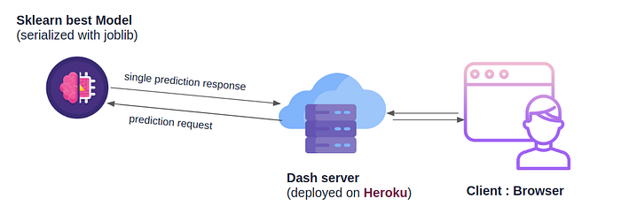
Our Dash uses Flask server under the hood, and will be deployed on heroku platform that supports Flask based apps. Once deployed the server would interact with our sklearn pre-trained model to update the prediction.
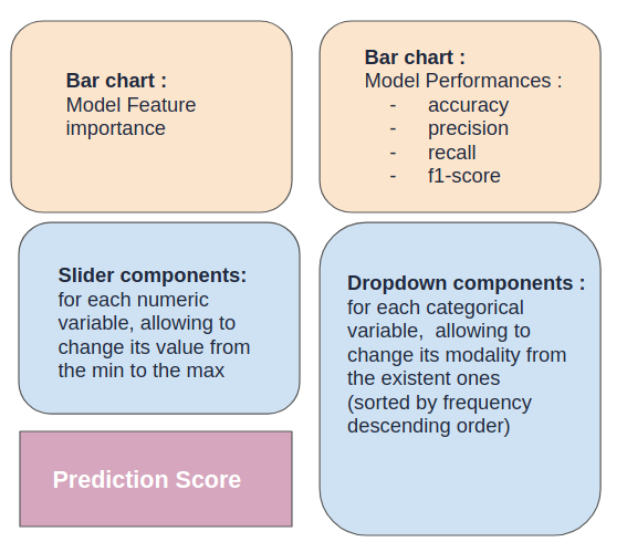
Now we have to design and implement the manner of how the dynamic elements will be displayed on our web browser.
For simplicity, we opted to create the app as follows (it can be improved):
import os
# We start with the import of standard ML librairies
import pandas as pd
import math
from joblib import load
from src.data_processing import make_full_pipeline
import pickle
# We add all Plotly and Dash necessary librairies
import dash
import plotly.graph_objects as go
import dash_core_components as dcc
import dash_html_components as html
from dash.dependencies import Input, Output

HOME_PATH = os.getcwd()
DATA_PATH = os.path.join(HOME_PATH, 'data')
MODELS_PATH = os.path.join(HOME_PATH, 'model')

df = pd.read_csv(os.path.join(DATA_PATH, "Customer-Value-Analysis.csv")).set_index('Customer')
sk_best = load(os.path.join(MODELS_PATH, 'best.joblib'))

# full_pipeline = load(os.path.join(MODELS_PATH, 'transformer.joblib'))
full_pipeline = make_full_pipeline(df)

ohe_path = os.path.join(MODELS_PATH, 'ohe_categories.pkl')
perfs_path = os.path.join(MODELS_PATH, 'sk_best_performances.pkl')

with open(ohe_path, 'rb') as input:
    ohe_categories = pickle.load(input)

categories = []
for k, l in ohe_categories.items():
    categories.append([f'{k}_{cat}' for cat in list(l)])
flatten = lambda l: [item for sublist in l for item in sublist]
categories = flatten(categories)

with open(perfs_path, 'rb') as input:
    perfs = pickle.load(input)
# scaling

cats = [var for var, var_type in df.dtypes.items() if var_type == 'object']
nums = [var for var in df.columns if var not in cats]
cats.remove('Response')

TOP = 10
# We create a DataFrame to store the features' importance and their corresponding label
df_feature_importances = pd.DataFrame(sk_best.feature_importances_ * 100, columns=["Importance"],
                                      index=nums + categories)
df_feature_importances = df_feature_importances.sort_values("Importance", ascending=False)
df_feature_importances = df_feature_importances.loc[df_feature_importances.index[:TOP]]

# We create a Features Importance Bar Chart
fig_features_importance = go.Figure()
fig_features_importance.add_trace(go.Bar(x=df_feature_importances.index,
                                         y=df_feature_importances["Importance"],
                                         marker_color='rgb(171, 226, 251)')
                                  )
fig_features_importance.update_layout(title_text='<b>Features Importance of the model<b>', title_x=0.5)

# We create a Features perfomances Bar Chart
fig_perfs = go.Figure()
fig_perfs.add_trace(go.Bar(y=list(perfs.keys()),
                           x=list(perfs.values()),
                           marker_color='rgb(171, 226, 251)',
                           orientation='h')
                    )
fig_perfs.update_layout(title_text='<b>Best Model Performances<b>', title_x=0.5)

cat_children = []
for var in cats:
    # Categorical children
    sorted_modalities = list(df[var].value_counts().index)
    cat_children.append(html.H4(children=var))
    cat_children.append(dcc.Dropdown(
        id='{}-dropdown'.format(var),
        options=[{'label': value, 'value': value} for value in sorted_modalities],
        value=sorted_modalities[0]
    ))

linear_children = []
for var in nums:
    # linear children
    linear_children.append(html.H4(children=var))
    desc = df[var].describe()
    linear_children.append(dcc.Slider(
        id='{}-dropdown'.format(var),
        min=math.floor(desc['min']),
        max=round(desc['max']),
        step=None,
        value=round(desc['mean']),
        marks={i: '{}°'.format(i) for i in
               range(int(desc['min']), int(desc['max']) + 1, max(int((desc['std'] / 1.5)), 1))}
    ))
This requires some explanations:
- To get the the feature importance corresponding to our model, we used the
feature_importances_attribute of thesk_bestmodel (found after fine tuning the random forest model in the previous step). - We retrieve the previously saved performances on
perfsdictionary variable that will be displayed as an horizontal bar chat - For every numerical feature we create its corresponding Slider element
- For each numerical feature we constructed a dropdown elementt
Now all we have to do is to is to combine the created HTML elements within the app principle layout:
app = dash.Dash(__name__,
# external CSS stylesheets
 external_stylesheets = [
     #"https://raw.githack.com/Athena75/IBM-Customer-Value-Dashboarding/main/assets/style.css",
     "https://rawcdn.githack.com/Athena75/IBM-Customer-Value-Dashboarding/df971ae38117d85c8512a72643ce6158cde7a4eb/assets/style.css"
 ]
)

# We apply basic HTML formatting to the layout
app.layout = html.Div(children=[
    # first row : Title
    html.Div(children=[
        html.Div(children=[html.H1(children="Simulation Tool : IBM Customer Churn")],
                 className='title'),

    ],
        style={"display": "block"}),
    # second row :
    html.Div(children=[
        # first column : fig feature importance + linear + prediction
        html.Div(children=[
            html.Div(children=[dcc.Graph(figure=fig_features_importance, className='graph')] + linear_children),
            # prediction result
            html.Div(children=[html.H2(children="Prediction:"),
                               html.H2(id="prediction_result")],
                     className='prediction')],
                 className='column'),
        # second column : fig performances categorical
        html.Div(children=[dcc.Graph(figure=fig_perfs, className='graph')] + cat_children,
                 className='column')
    ],
        className='row')
]
)
The classNameelements refers to CSS classes that are defined in this gist.
The CSS link must be settled in external_stylesheets parameter so that the dash app knows that it will include the css from an external resource (I borrowed the idea from here).
Please note that this part has taken me a looot of time that I want you to save. As shown above, Dash allows you to import external css resources. The question is how to create your own css resources and make them exploitable. Well, one solution consists in saving it on a gist within your github profile. However when you would request your gist, the response is usually served with a Content-Type=text/plain. As a result, your browser won’t actually interpret it as a CSS type.
The solution consists on passing the related url to the raw.githack.com proxy allowing to relay the app requests with the correct Content-Type header.
I hosted the css gist within /assets/style.css inside my github root project then I changed it via the raw.github proxy:
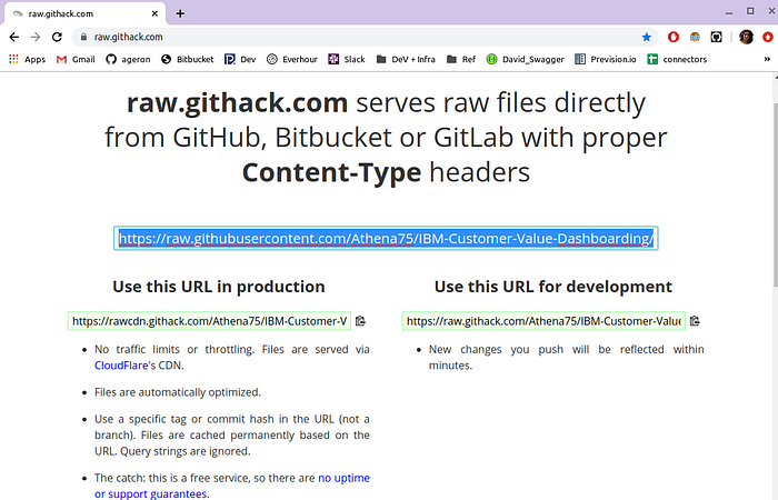
I retrieved the production URL and added it into theexternal_stylesheets dash app parameter.
Let’s get back to our dash app: In the previous code snippet, you can notice that I added a new html division with id=prediction_result ; it will be used to identify the related HTML element (our score text) to update it in a dynamic manner. So we need to make the different HTML components interact with each other.
Dash makes it possible via the app.callback functions: We will implement a callback function that changes dynamically the HTML element identified by prediction_result every time the value of the other elements change, without having to reloading the page:
# The callback function will provide one "Output" in the form of a string (=children)
@app.callback(Output(component_id="prediction_result", component_property="children"),
              # The values corresponding to sliders and dropdowns of respectively numerical and categorical features
              [Input('{}-dropdown'.format(var), 'value') for var in nums + cats])
# The input variable are set in the same order as the callback Inputs
def update_prediction(*X):
    # get the data input and map it to the correponding feature names
    payload = dict(zip(nums + cats, X))
    # create one line dataframe
    frame_X = pd.DataFrame(payload, index=[0])
    # pass it through the pre-fitted transformer
    X_processed = full_pipeline.transform(frame_X)

    prediction = sk_best.predict_proba(X_processed)[0]

    # And retuned to the Output of the callback function
    return " {}% No , {}% Yes".format("%.2f" % (prediction[0] * 100),
                                      "%.2f" % (prediction[1] * 100))
To test out your code, add a run.py script inside your root project folder and add :
from src.app_dash import server
With dash_app.py the dash app script you can find it here
Then you can either use the Flask server (packaged by the Dash app) or gunicorn (which is recommended)
With gunicorn :
$gunicorn run:server
Deploy on heroku:
To succeed your deployment on Heroku you have to provide within your root project repos two special files:
- Procfile: It gives the instructions to execute when starting the application.
web: gunicorn run:server
- requirements.txt: lists the libraries to install: To get all the required packages for your project you can use this command:
pip freeze > requirements.txt
Before using heroku you have to commit all changes to your github repo
- Install:
First of all you have to install heroku : according to your OS install it as described here: https://devcenter.heroku.com/articles/heroku-cli
2. Create a new heroku app:
Example:
$heroku create ibm-customer-churn-simulator
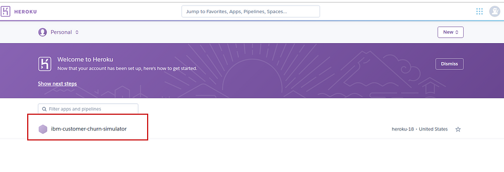
3. Connect your app to your Github repos:
Now that the new app is created all we have to do is to connect it to our github repo, click on it, go to the Deploy tab and choose Github in the Deployment method section :
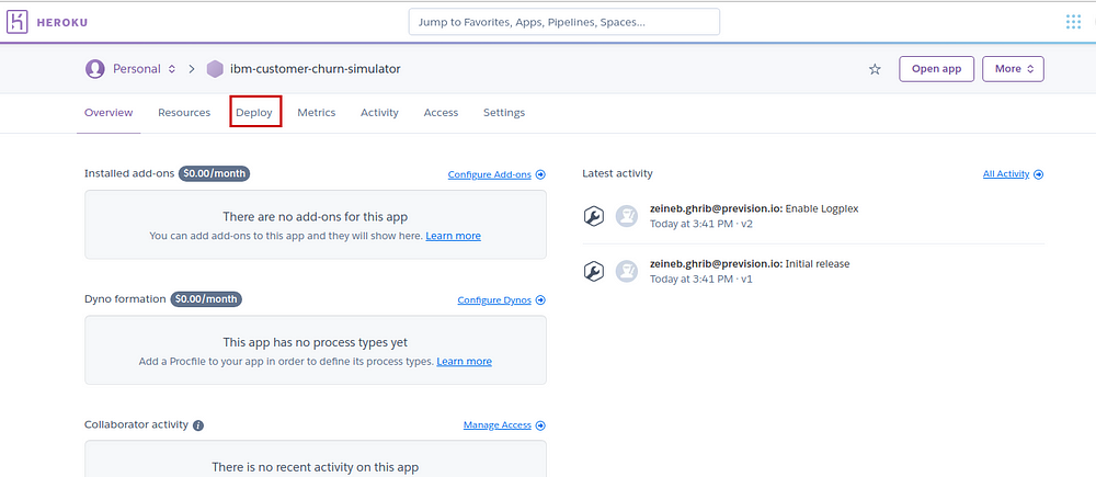
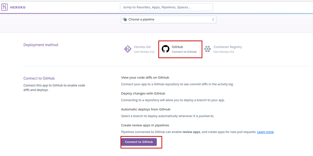
Then select your repository and the corresponding branch.
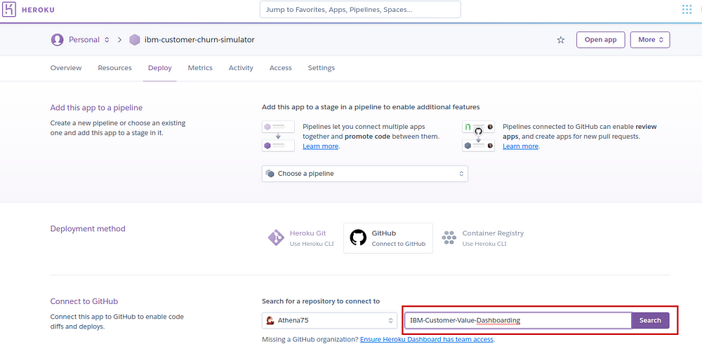
Finally, click on Deploy Branch Button
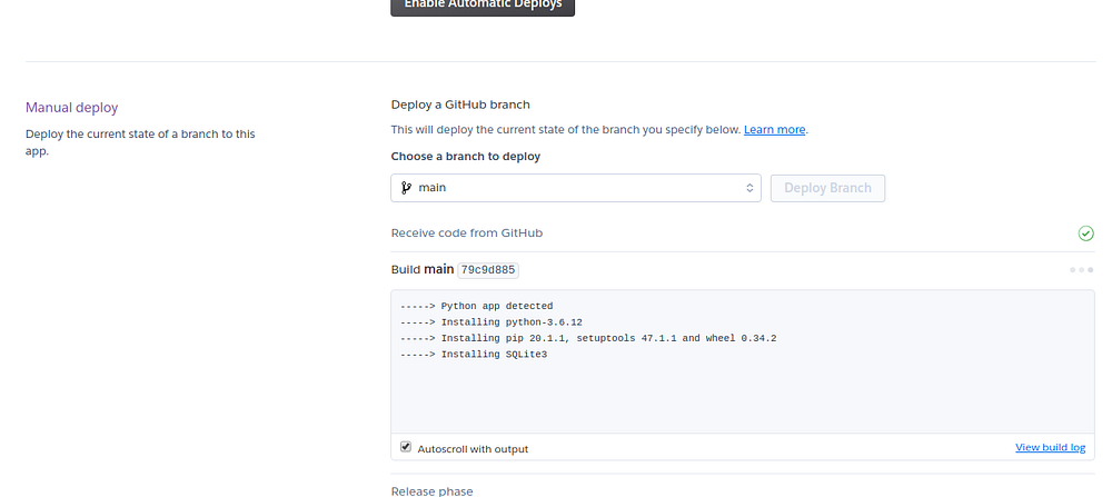
Now starts the stressful moment :///…… Wait for deployment success!!!
If everything goes well, you get this green message:
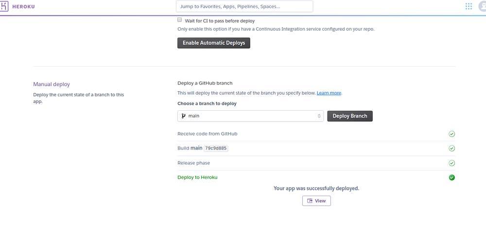
And finally you get your app :
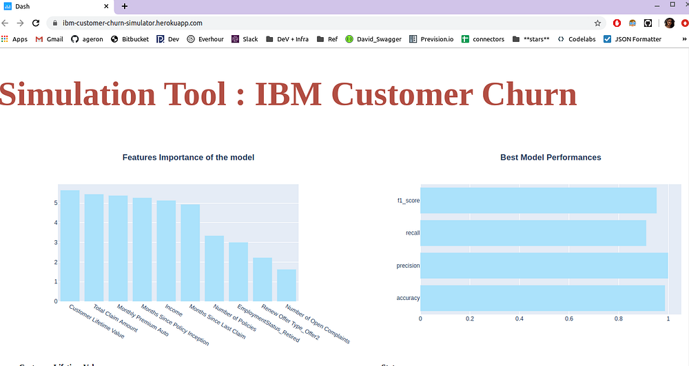
Here the link to the app, hosted on heroku.
This article has been published from the source link without modifications to the text. Only the headline has been changed.
Source link


