Create a Similarity Measure
- Create a Manual Similarity Measure
- Supervised Similarity Measure
- Generating Embeddings Example
- Measuring Similarity from Embeddings
- Supervised Similarity Calculation: Programming Exercise
- Similarity Measures: Check Your Understanding
- Similarity Measure Summary
- Run the Clustering Algorithm
- Interpret Results and Adjust Clustering
- k-Means Advantages and Disadvantages
Create a Manual Similarity Measure
To calculate the similarity between two examples, you need to combine all the feature data for those two examples into a single numeric value.
For instance, consider a shoe data set with only one feature: shoe size. You can quantify how similar two shoes are by calculating the difference between their sizes. The smaller the numerical difference between sizes, the greater the similarity between shoes. Such a handcrafted similarity measure is called a manual similarity measure.
What if you wanted to find similarities between shoes by using both size and color? Color is categorical data, and is harder to combine with the numerical size data. We will see that as data becomes more complex, creating a manual similarity measure becomes harder. When your data becomes complex enough, you won’t be able to create a manual measure. That’s when you switch to a supervised similarity measure, where a supervised machine learning model calculates the similarity.
We’ll leave the supervised similarity measure for later and focus on the manual measure here. For now, remember that you switch to a supervised similarity measure when you have trouble creating a manual similarity measure.
To understand how a manual similarity measure works, let’s look at our example of shoes. Suppose the model has two features: shoe size and shoe price data. Since both features are numeric, you can combine them into a single number representing similarity as follows.
- Size (s): Shoe size probably forms a Gaussian distribution. Confirm this. Then normalize the data.
- Price (p): The data is probably a Poisson distribution. Confirm this. If you have enough data, convert the data to quantiles and scale to [0,1].
- Combine the data by using root mean squared error (RMSE). Here, the similarity is

For a simplified example, let’s calculate similarity for two shoes with US sizes 8 and 11, and prices 120 and 150. Since we don’t have enough data to understand the distribution, we’ll simply scale the data without normalizing or using quantiles.
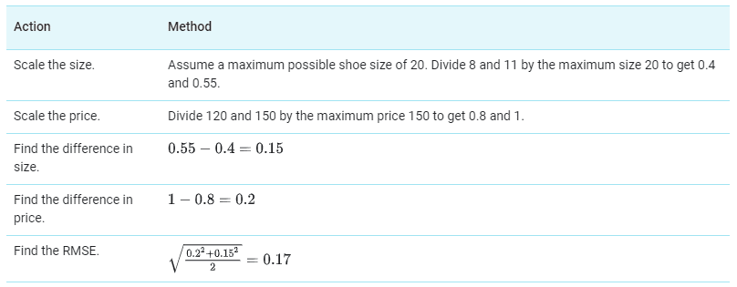
Intuitively, your measured similarity should increase when feature data becomes similar. Instead, your measured similarity actually decreases. Make your measured similarity follow your intuition by subtracting it from 1.
Similarity=1−0.17=0.83
In general, you can prepare numerical data as described in Prepare data, and then combine the data by using Euclidean distance.
What if you have categorical data? Categorical data can either be:
- Single valued (univalent), such as a car’s color (“white” or “blue” but never both)
- Multi-valued (multivalent), such as a movie’s genre (can be “action” and “comedy” simultaneously, or just “action”)
If univalent data matches, the similarity is 1; otherwise, it’s 0. Multivalent data is harder to deal with. For example, movie genres can be a challenge to work with. To handle this problem, suppose movies are assigned genres from a fixed set of genres. Calculate similarity using the ratio of common values, called Jaccard similarity.
Examples:
- [“comedy”,”action”] and [“comedy”,”action”] = 1
- [“comedy”,”action”] and [“action”] = ½
- [“comedy”,”action”] and [“action”, “drama”] = ⅓
- [“comedy”,”action”] and [“non-fiction”,”biographical”] = 0
The following table provides a few more examples of how to deal with categorical data.

In general, your similarity measure must directly correspond to the actual similarity. If your metric does not, then it isn’t encoding the necessary information. The preceding example converted postal codes into latitude and longitude because postal codes by themselves did not encode the necessary information.
Before creating your similarity measure, process your data carefully. Although the examples on this page relied on a small, simple data set, most real-world data sets are far bigger and far more complex. Remember that quantiles are a good default choice for processing numeric data.
Supervised Similarity Measure
Instead of comparing manually-combined feature data, you can reduce the feature data to representations called embeddings, and then compare the embeddings. Embeddings are generated by training a supervised deep neural network (DNN) on the feature data itself. The embeddings map the feature data to a vector in an embedding space. Typically, the embedding space has fewer dimensions than the feature data in a way that captures some latent structure of the feature data set. The embedding vectors for similar examples, such as YouTube videos watched by the same users, end up close together in the embedding space. We will see how the similarity measure uses this “closeness” to quantify the similarity for pairs of examples.
Remember, we’re discussing supervised learning only to create our similarity measure. The similarity measure, whether manual or supervised, is then used by an algorithm to perform unsupervised clustering.
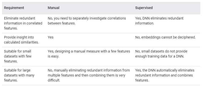
Comparison of Manual and Supervised Measures
This table describes when to use a manual or supervised similarity measure depending on your requirements.
Process for Supervised Similarity Measure
The following figure shows how to create a supervised similarity measure:

You’ve already learned the first step. This page discusses the next step, and the following pages discuss the remaining steps.
Choose DNN Based on Training Labels
Reduce your feature data to embeddings by training a DNN that uses the same feature data both as input and as the labels. For example, in the case of house data, the DNN would use the features—such as price, size, and postal code—to predict those features themselves. In order to use the feature data to predict the same feature data, the DNN is forced to reduce the input feature data to embeddings. You use these embeddings to calculate similarity.
A DNN that learns embeddings of input data by predicting the input data itself is called an autoencoder. Because an autoencoder’s hidden layers are smaller than the input and output layers, the autoencoder is forced to learn a compressed representation of the input feature data. Once the DNN is trained, you extract the embeddings from the last hidden layer to calculate similarity.

An autoencoder is the simplest choice to generate embeddings. However, an autoencoder isn’t the optimal choice when certain features could be more important than others in determining similarity. For example, in house data, let’s assume “price” is more important than “postal code”. In such cases, use only the important feature as the training label for the DNN. Since this DNN predicts a specific input feature instead of predicting all input features, it is called a predictor DNN. Use the following guidelines to choose a feature as the label:
- Prefer numeric features to categorical features as labels because loss is easier to calculate and interpret for numeric features.
- Do not use categorical features with cardinality ≲ 100 as labels. If you do, the DNN will not be forced to reduce your input data to embeddings because a DNN can easily predict low-cardinality categorical labels.
- Remove the feature that you use as the label from the input to the DNN; otherwise, the DNN will perfectly predict the output.
Depending on your choice of labels, the resulting DNN is either an autoencoder DNN or a predictor DNN.
Loss Function for DNN
To train the DNN, you need to create a loss function by following these steps:
- Calculate the loss for every output of the DNN. For outputs that are:
- Numeric, use mean square error (MSE).
- Univalent categorical, use log loss. Note that you won’t need to implement log loss yourself because you can use a library function to calculate it.
- Multivalent categorical, use softmax cross entropy loss. Note that you won’t need to implement softmax cross entropy loss yourself because you can use a library function to calculate it.
- Calculate the total loss by summing the loss for every output.
When summing the losses, ensure that each feature contributes proportionately to the loss. For example, if you convert color data to RGB values, then you have three outputs. But summing the loss for three outputs means the loss for color is weighted three times as heavily as other features. Instead, multiply each output by 1/3.
Using DNN in an Online System
An online machine learning system has a continuous stream of new input data. You’ll need to train your DNN on the new data. However, if you retrain your DNN from scratch, then your embeddings will be different because DNNs are initialized with random weights. Instead, always warm-start the DNN with the existing weights and then update the DNN with new data.
Generating Embeddings Example
This example shows how to generate the embeddings used in a supervised similarity measure.
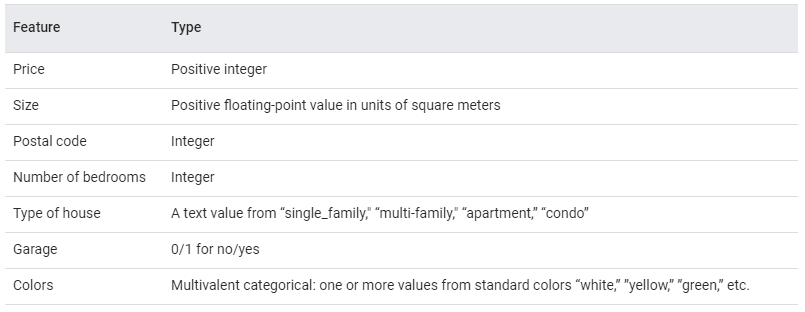
Imagine you have the same housing data set that you used when creating a manual similarity measure:
Preprocessing Data
Before you use feature data as input, you need to preprocess the data. The preprocessing steps are based on the steps you took when creating a manual similarity measure. Here’s a summary:
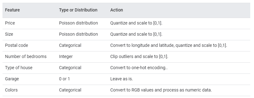
For more information on one-hot encoding, see Embeddings: Categorical Input Data.
Choose Predictor or Autoencoder
To generate embeddings, you can choose either an autoencoder or a predictor. Remember, your default choice is an autoencoder. You choose a predictor instead if specific features in your dataset determine similarity. For completeness, let’s look at both cases.
Train a Predictor
You need to choose those features as training labels for your DNN that are important in determining similarity between your examples. Let’s assume price is most important in determining similarity between houses.
Choose price as the training label, and remove it from the input feature data to the DNN. Train the DNN by using all other features as input data. For training, the loss function is simply the MSE between predicted and actual price. To learn how to train a DNN, see Training Neural Networks.
Train an Autoencoder
Train an autoencoder on our dataset by following these steps:
- Ensure the hidden layers of the autoencoder are smaller than the input and output layers.
- Calculate the loss for each output as described in Supervised Similarity Measure.
- Create the loss function by summing the losses for each output. Ensure you weight the loss equally for every feature. For example, because color data is processed into RGB, weight each of the RGB outputs by 1/3rd.
- Train the DNN.
Extracting Embeddings from the DNN
After training your DNN, whether predictor or autoencoder, extract the embedding for an example from the DNN. Extract the embedding by using the feature data of the example as input, and read the outputs of the final hidden layer. These outputs form the embedding vector. Remember, the vectors for similar houses should be closer together than vectors for dissimilar houses.
Next, you’ll see how to quantify the similarity for pairs of examples by using their embedding vectors.
Measuring Similarity from Embeddings
You now have embeddings for any pair of examples. A similarity measure takes these embeddings and returns a number measuring their similarity. Remember that embeddings are simply vectors of numbers. To find the similarity between two vectors

and

you have three similarity measures to choose from, as listed in the table below.
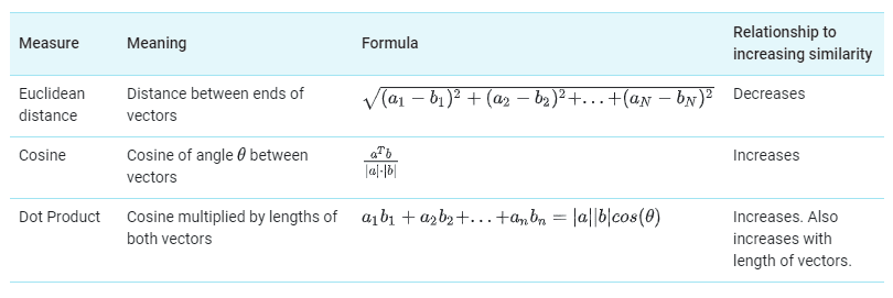
Choosing a Similarity Measure
In contrast to the cosine, the dot product is proportional to the vector length. This is important because examples that appear very frequently in the training set (for example, popular YouTube videos) tend to have embedding vectors with large lengths. If you want to capture popularity, then choose dot product. However, the risk is that popular examples may skew the similarity metric. To balance this skew, you can raise the length to an exponent

to calculate the dot product as

To better understand how vector length changes the similarity measure, normalize the vector lengths to 1 and notice that the three measures become proportional to each other.

Supervised Similarity Calculation: Programming Exercise
Estimated Time: 15 minutes
This Colab shows how to design a supervised similarity measure for a dataset of chocolate bar ratings. You will do the following:
- Load and clean the data.
- Inspect and prepare the data.
- Generate embeddings for chocolate data using a DNN.
Note: Complete only sections 1, 2, and 3. We will return to sections 4 and 5 after studying the k-means algorithm and quality metrics.
Similarity Measures: Check Your Understanding

In the image above, if you want “b” to be more similar to “a” than “b” is to “c”, which measure should you pick?
Euclidean distance
Dot product
Cosine
Correct answer:
Dot product – The dot product is proportional to both the cosine and the lengths of vectors. So even though the cosine is higher for “b” and “c”, the higher length of “a” makes “a” and “b” more similar than “b” and “c”.
You are calculating similarity for music videos. The length of the embedding vectors of music videos is proportional to their popularity. You now choose dot product instead of cosine to calculate similarity. How does similarity between music videos change?
Popular videos become less similar than less popular videos.
Popular videos become more similar to all videos in general.
No change.
Correct answer:
Popular videos become more similar to all videos in general –
Since the dot product is affected by the lengths of both vectors, the large vector length of popular videos will make them more similar to all videos.
In the same scenario as the previous question, suppose you switch to cosine from dot product. How does similarity between music videos change?
No change.
Popular videos become more similar than less popular videos.
Popular videos become less similar than less popular videos.
Correct answer:
Popular videos become less similar than less popular videos –
Because cosine is not affected by vector length, the large vector length of embeddings of popular videos does not contribute to similarity. Thus, switching to cosine from dot product reduces the similarity for popular videos.
Similarity Measure Summary
To summarize, a similarity measure quantifies the similarity between a pair of examples, relative to other pairs of examples. The table below compares the two types of similarity measures:

Run the Clustering Algorithm
In machine learning, you sometimes encounter datasets that can have millions of examples. ML algorithms must scale efficiently to these large datasets. However, many clustering algorithms do not scale because they need to compute the similarity between all pairs of points. This means their runtimes increase as the square of the number of points, denoted as

For example, agglomerative or divisive hierarchical clustering algorithms look at all pairs of points and have complexities of

and

This course focuses on k-means because it scales as O(nk), where k is the number of clusters. k-means groups points into k clusters by minimizing the distances between points and their cluster’s centroid (as seen in Figure 1 below). The centroid of a cluster is the mean of all the points in the cluster.
As shown, k-means finds roughly circular clusters. Conceptually, this means k-means effectively treats data as composed of a number of roughly circular distributions, and tries to find clusters corresponding to these distributions. In reality, data contains outliers and might not fit such a model.
Before running k-means, you must choose the number of clusters, k. Initially, start with a guess for k. Later, we’ll discuss how to refine this number.
k-means Clustering Algorithm
To cluster data into k clusters, k-means follows the steps below:

Step One
The algorithm randomly chooses a centroid for each cluster. In our example, we choose a k of 3, and therefore the algorithm randomly picks 3 centroids.

Step Two
The algorithm assigns each point to the closest centroid to get k initial clusters.

Step Three
For every cluster, the algorithm recomputes the centroid by taking the average of all points in the cluster. The changes in centroids are shown in Figure 3 by arrows. Since the centroids change, the algorithm then re-assigns the points to the closest centroid. Figure 4 shows the new clusters after re-assignment.

Step Four
The algorithm repeats the calculation of centroids and assignment of points until points stop changing clusters. When clustering large datasets, you stop the algorithm before reaching convergence, using other criteria instead.
You do not need to understand the math behind k-means for this course. However, if you are curious, see below for the mathematical proof.
Because the centroid positions are initially chosen at random, k-means can return significantly different results on successive runs. To solve this problem, run k-means multiple times and choose the result with the best quality metrics. (We’ll describe quality metrics later in this course.) You’ll need an advanced version of k-means to choose better initial centroid positions.
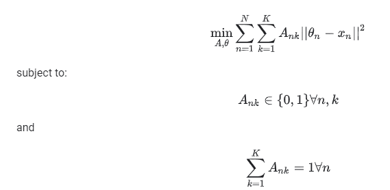
Given n examples assigned to k clusters, minimize the sum of distances of examples to their centroids. Where:

nth example is assigned to the
kth cluster, and 0 otherwise

We want to minimize the following expression:
To minimize the expression with respect to the cluster centroids

take the derivative with respect to

and equate it to 0.
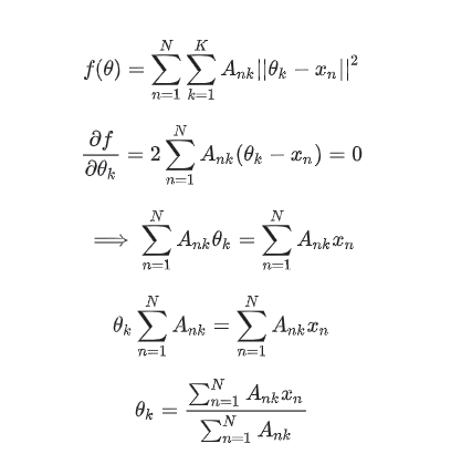
The numerator is the sum of all example-centroid distances in the cluster. The denominator is the number of examples in the cluster. Thus, the cluster centroid θk is the average of example-centroid distances in the cluster. Hence proved.
Because the centroid positions are initially chosen at random, k-means can return significantly different results on successive runs. To solve this problem, run k-means multiple times and choose the result with the best quality metrics. (We’ll describe quality metrics later in this course.) You’ll need an advanced version of k-means to choose better initial centroid positions.
Experiment: Using this k-means simulator from Stanford, try running k-means multiple times and see if you get different results.
Interpret Results and Adjust Clustering
Because clustering is unsupervised, no “truth” is available to verify results. The absence of truth complicates assessing quality. Further, real-world datasets typically do not fall into obvious clusters of examples like the dataset shown in Figure 1.
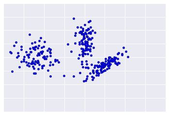
Sadly, real-world data looks more like Figure 2, making it difficult to visually assess clustering quality.
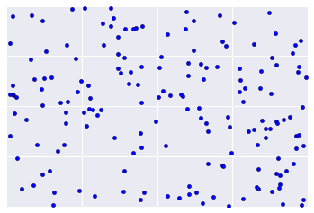
The flowchart below summarizes how to check the quality of your clustering. We’ll expand upon the summary in the following sections.

Step One: Quality of Clustering
Checking the quality of clustering is not a rigorous process because clustering lacks “truth”. Here are guidelines that you can iteratively apply to improve the quality of your clustering.
First, perform a visual check that the clusters look as expected, and that examples that you consider similar do appear in the same cluster. Then check these commonly-used metrics as described in the following sections:
- Cluster cardinality
- Cluster magnitude
- Performance of downstream system
Note: While several other metrics exist to evaluate clustering quality, these three metrics are commonly-used and beneficial.
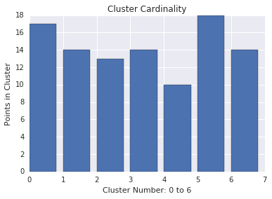
Cluster cardinality
Cluster cardinality is the number of examples per cluster. Plot the cluster cardinality for all clusters and investigate clusters that are major outliers. For example, in Figure 2, investigate cluster number 5.
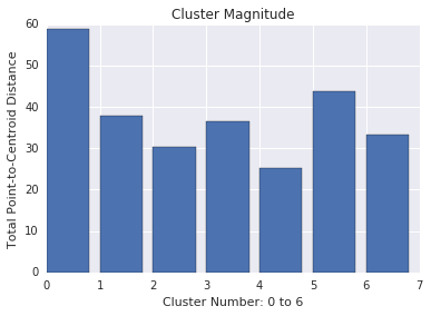
Cluster magnitude
Cluster magnitude is the sum of distances from all examples to the centroid of the cluster. Similar to cardinality, check how the magnitude varies across the clusters, and investigate anomalies. For example, in Figure 3, investigate cluster number 0.

Magnitude vs. Cardinality
Notice that a higher cluster cardinality tends to result in a higher cluster magnitude, which intuitively makes sense. Clusters are anomalous when cardinality doesn’t correlate with magnitude relative to the other clusters. Find anomalous clusters by plotting magnitude against cardinality. For example, in Figure 4, fitting a line to the cluster metrics shows that cluster number 0 is anomalous.
Performance of Downstream System
Since clustering output is often used in downstream ML systems, check if the downstream system’s performance improves when your clustering process changes. The impact on your downstream performance provides a real-world test for the quality of your clustering. The disadvantage is that this check is complex to perform.
Questions to Investigate If Problems are Found
If you find problems, then check your data preparation and similarity measure, asking yourself the following questions:
- Is your data scaled?
- Is your similarity measure correct?
- Is your algorithm performing semantically meaningful operations on the data?
- Do your algorithm’s assumptions match the data?
Step Two: Performance of the Similarity Measure
Your clustering algorithm is only as good as your similarity measure. Make sure your similarity measure returns sensible results. The simplest check is to identify pairs of examples that are known to be more or less similar than other pairs. Then, calculate the similarity measure for each pair of examples. Ensure that the similarity measure for more similar examples is higher than the similarity measure for less similar examples.
The examples you use to spot check your similarity measure should be representative of the data set. Ensure that your similarity measure holds for all your examples. Careful verification ensures that your similarity measure, whether manual or supervised, is consistent across your dataset. If your similarity measure is inconsistent for some examples, then those examples will not be clustered with similar examples.
If you find examples with inaccurate similarities, then your similarity measure probably does not capture the feature data that distinguishes those examples. Experiment with your similarity measure and determine whether you get more accurate similarities.
Step Three: Optimum Number of Clusters
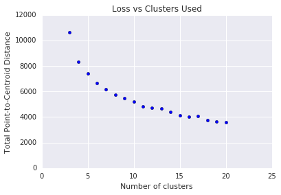
k-means requires you to decide the number of clusters k beforehand. How do you determine the optimal value of k? Try running the algorithm for increasing k and note the sum of cluster magnitudes. As k increases, clusters become smaller, and the total distance decreases. Plot this distance against the number of clusters.
As shown in Figure 4, at a certain k, the reduction in loss becomes marginal with increasing k. Mathematically, that’s roughly the k where the slope crosses above

This guideline doesn’t pinpoint an exact value for the optimum k but only an approximate value. For the plot shown, the optimum k is approximately 11. If you prefer more granular clusters, then you can choose a higher k using this plot as guidance.
k-Means Advantages and Disadvantages
Advantages of k-means
Relatively simple to implement.
Scales to large data sets.
Guarantees convergence.
Can warm-start the positions of centroids.
Easily adapts to new examples.
Generalizes to clusters of different shapes and sizes, such as elliptical clusters.
k-means Generalization
What happens when clusters are of different densities and sizes? Look at Figure 1. Compare the intuitive clusters on the left side with the clusters actually found by k-means on the right side. The comparison shows how k-means can stumble on certain datasets.

To cluster naturally imbalanced clusters like the ones shown in Figure 1, you can adapt (generalize) k-means. In Figure 2, the lines show the cluster boundaries after generalizing k-means as:
- Left plot: No generalization, resulting in a non-intuitive cluster boundary.
- Center plot: Allow different cluster widths, resulting in more intuitive clusters of different sizes.
- Right plot: Besides different cluster widths, allow different widths per dimension, resulting in elliptical instead of spherical clusters, improving the result.

While this course doesn’t dive into how to generalize k-means, remember that the ease of modifying k-means is another reason why it’s powerful. For information on generalizing k-means, see Clustering – K-means Gaussian mixture models by Carlos Guestrin from Carnegie Mellon University.
Disadvantages of k-means
Choosing k manually.
Use the “Loss vs. Clusters” plot to find the optimal (k), as discussed in Interpret Results.
Being dependent on initial values.
For a low k, you can mitigate this dependence by running k-means several times with different initial values and picking the best result. As k increases, you need advanced versions of k-means to pick better values of the initial centroids (called k-means seeding). For a full discussion of k– means seeding see, A Comparative Study of Efficient Initialization Methods for the K-Means Clustering Algorithm by M. Emre Celebi, Hassan A. Kingravi, Patricio A. Vela.
Clustering data of varying sizes and density.
k-means has trouble clustering data where clusters are of varying sizes and density. To cluster such data, you need to generalize k-means as described in the Advantages section.
Clustering outliers.
Centroids can be dragged by outliers, or outliers might get their own cluster instead of being ignored. Consider removing or clipping outliers before clustering.
Scaling with number of dimensions.
As the number of dimensions increases, a distance-based similarity measure converges to a constant value between any given examples. Reduce dimensionality either by using PCA on the feature data, or by using “spectral clustering” to modify the clustering algorithm as explained below.
Curse of Dimensionality and Spectral Clustering
These plots show how the ratio of the standard deviation to the mean of distance between examples decreases as the number of dimensions increases. This convergence means k-means becomes less effective at distinguishing between examples. This negative consequence of high-dimensional data is called the curse of dimensionality.

Spectral clustering avoids the curse of dimensionality by adding a pre-clustering step to your algorithm:
- Reduce the dimensionality of feature data by using PCA.
- Project all data points into the lower-dimensional subspace.
- Cluster the data in this subspace by using your chosen algorithm.
Therefore, spectral clustering is not a separate clustering algorithm but a pre- clustering step that you can use with any clustering algorithm.
[ad_2]
This article has been published from the source link without modifications to the text. Only the headline has been changed.


