Building an efficient data model in Power BI

Power BI is one of the leading data visualisation tools on the market. This current article is part of the Power BI like a Pro series written by TrueCue’s most experienced Power BI developers.

This series’ objective is to walk users through the main considerations and strategies to build enterprise level Power BI reporting solutions.

The following article will show how to create an efficient Power BI data model, the basis of any type of Power BI development.

Power BI is one of the only data visualisation platforms allowing analysts to create a data model at the backend of a report. With Power BI, data can be drawn from many different sources (database, Excel, Python/R script…) and joined up within the report itself!

This great power implies great responsibilities, as decisions taken in the data modelling process will have a significant influence on the report’s fitness for purpose and efficiency.

Data Modelling Basics

Before diving into the intricacies of Power BI data modelling, it is critical to understand some basic data modelling concepts.

A data model can be defined as the organisation and relationships of a set of two or more data tables.

There are several ways to represent data models, one of the most commonly used method is the Entity-Relationship Diagram (ERD).

Power BI’s data model view represents the report’s data model with an ERD:

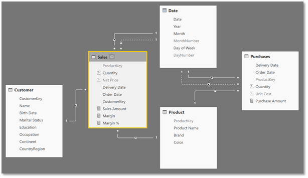
In Power BI, developers can access the “Data Model” view by clicking on this icon on the left pane of the Power BI Desktop interface:

Data models are central to relational databases and data warehouses. They describe how different tables are linked to one another. The goal of the data modelling process is to design the optimal data architecture/relationships for a specific purpose. It is important to note that even if there exist data model best practices, the one-size-fits-all data model is still to be discovered.

As its name indicates, traditional entity-relationship models are composed of two key elements:

1. Data Tables (“entities”)

A data table can be conceptualised as a way to store information in a tabular format, with rows and columns (see the diagram below):

Each row is a particular instance, observation, or entity-type. Each column is an attribute. A single row of data has several attributes. As an example, the row highlighted in the example table above is a meteorological observation of the 23/08/2020. This observation has several attributes (“columns”), including temperature, humidity and precipitations.

2. Data Relationships (“relationships”)

A data relationship is the way in which different data tables are linked together. In other word, it describes the way in which the information stored in one table relates to the information stored in another. The following simple example will illustrate the concept of data relationships:

Let’s consider two tables:

• Fact_Sales: recording daily sales volume for each product
• Dim_Product: storing product information such as name and description

These two tables are linked by “Product ID”. In practice, this means that the product information can be accessed from sales through the “Product ID” attribute. In other words, retrieving the product names that have sold the greatest quantity will require a search through Product IDs in the Fact_Sales table, and a join with Dim_Product to retrieve the product names of the highest selling Product IDs.

The relationship key is the field used to travel from one table to the next, i.e. to link information stored in two different tables.

This relationship between Fact_Sales and Dim_Product has a many-to-one cardinality. This means that each row into the Product Information table (Dim_Product) links to several rows in the Product Sales table (Fact_Sales). In other word, a single product ID, is featured several times in the Sales Table, and only once in the Product Information table.

A data relationship’s cardinality describes the numerical relationship between rows of one table and the rows of the other. The main cardinalities include:

• one-to-one: one-to-one cardinality indicates that each row of a table maps to a single row of another table
• one-to-many (or “many-to-one”): one-to-many relationships are very frequent in traditional star-schemas. One-to-many relationships occur when a single row of a table maps to more than one row in another table. This is the case of the example relationship studied above
• many-to-many: many-to-many relationships are very tricky to deal with. They occur when multiple rows in one table link to multiple rows in another

Now that the main data-modelling concepts have been defined, the following sections will go through the design of an efficient data model in Power BI.

Data Modelling Decisions in Power BI

Designing a Power BI data model can be viewed as a series of decisions. As in many cases in the world of analytics, despite the existence of best practices, the perfect data model or data architecture does not exist. The optimal data model will ultimately depend on the objective and constrained faced by analytics teams.

1. Import or Direct Query

The first question to answer when creating a Power BI data model is: How to connect to the different report data sources?

When connecting to a data source using the “Get Data” feature:

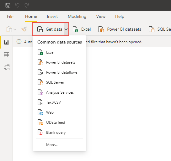
Power BI will usually give users the choice between “Import” and “Direct Query”:

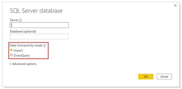
In summary, “Import” relies on caching data extracts, while “DirectQuery” maintains an active data connection between the report and the data sources, that will be queried at each visual interaction. The advantages and disadvantages of these two methods will be described in the section below.

Import

As explained above, “Import” connections create a copy of the data. This copy is cached on Power BI Desktop. Once the report is uploaded to Power BI service, the data extract will rest in Microsoft Data Services. This extract will be refreshed either on demand or on schedule, depending on the specific requirements of each use-case.

“Import” connections present several advantages:

1. Performance: As the data is cached, reports based on “Import” connections are usually much faster than their “DirectQuery” equivalents
2. Data Source Availability: Every data source supported by Power BI allows “Import” connections
3. DAX and Power Query Features: Reports working with “Import” connections can leverage all the available DAX and Power Query features.

Despite these significant advantages, “Import” connections still pose a few challenges:

1. Memory Limitations:

As “Import” connections create data extracts, they have a dataset size limit of 1GB. This ceiling can be pushed up to 10GB with certain premium options, but it still exists.

Note: On this specific point, there are many ways to reduce the size of a Power BI dataset, including pre-aggregated tables or optimising column data types.

2. Data Latency: As its name indicates, “Import” data connections are based on cached data extracts. This means that there could be latency between the data in the data sources and the data presented on the visuals. Depending on the use-cases, this could prove to be an issue.

“DirectQuery” connections were designed to address these two challenges.

Direct Query

In “DirectQuery” report, the schema and shape of the data is imported into Power BI but the data stays in the data source. Each visual interaction will query that data source. Thanks to this process Direct Query reports can efficiently deal with “Import”’s two main weaknesses:

1. Large Datasets: Because no data is cached in the reports, “DirectQuery” reports can efficiently deal with very large datasets, without having to worry about the storage ceilings imposed by “Import” connections.
2. Live Information: As each visual interaction queries the data source, Direct Query reports always display the data found in the data source at any point – no need to worry about refresh schedules.

Despite these two considerable strengths, Direct Query presents a few key weaknesses:

1. Performance: Many data sources are not set up to handle “DirectQuery” correctly, leading to important performance issues. Direct Query reports are difficult to set up and require a significant amount of performance testing.
2. Data Source Availability: Only a subset of Power BI data sources supports “DirectQuery”.
3. DAX and Power Query Capabilities: Several DAX and Power Query features, including date intelligence, are not available in “DirectQuery” reports. These advanced features would generate very long and slow SQL queries, which would be unsustainable in “DirectQuery” reporting.

Making the right connectivity choice

As shown above, there is no optimal connectivity mode. Both “Import” and “DirectQuery” present advantages and disadvantages. The right mode will ultimately depend on the use-case at hand and the requirements of a given solution.

General rule of thumb: Use “Import” when possible, switching to Direct Query when dealing with very large dataset or real-time reporting.

2. Data Processing

The second important question to answer when designing a Power BI data model is: How much of the data processing should be carried by the database? i.e. before the data is imported into Power BI.

In some cases, this is not even a question, as reports might have to be developed from static sources such as Excel spreadsheet or csv files. In these situations, the data processing work will have to be carried out in Power BI regardless.

When analysts have a reasonable level of control over their data sources, the general rule of thumb is that data processing should be pushed to the database as much as possible, leaving only aggregations to Power BI. This becomes even more important when the data size increases to millions of rows.

This can be done by creating SQL views in the data source database and pointing the Power BI report to these views. Without view creation permissions, data can also be imported using custom SQL Queries in Power BI.

All the data-processing made before and during import will not have to be carried out during report consumption, usually resulting in much faster reports.

3. Data Shape

Another important consideration is the shape of the data. The two traditional data shapes are “long” and “wide”. The example below shows how the same information can be stored in both a long and wide format:

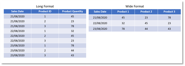
It is important to mention that a wide format can be used much more intuitively. Each of the columns is shown as a field in Power BI Desktop, and anyone could just drag this fields onto the canvas and start designing a report.

However, what if there were more than 300 different products? What if there was an unknown number of products? The flexibility of long format data addresses this issue. Long formats usually require more sophisticated calculations but open a wide range of visualisation possibilities.

Note: Data shape transformations should be processed upstream (in the database) as much as possible. However, if analysts do not have access to the database, the incoming data can always be pivoted within Power BI with Power Query or custom SQL queries.

4. Data Relationships

Once all the tables have been loaded into Power BI, they have to be linked correctly. This step involves setting up the relationships between the different data tables. The “Data Modelling Basics” section of this article covers the main concepts behind data relationships. This section will be mostly concerned with the implementation of these concepts in the Power BI Desktop interface.

This example will use the two tables (Fact_Sales and Dim_Product) shown in an earlier example and go through the process of loading them and linking them in Power BI:

These tables can be loaded into a blank Power BI report using either an Excel file and the “Get Data” feature, or the “Enter Data” feature (to type the data manually into Power BI)

Creating Data Relationships

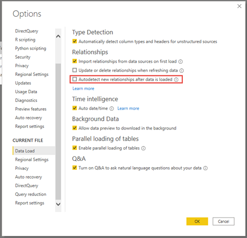
1. Loading these two tables into the report, Power BI could detect the relationships between these entities automatically. However, it is always better to review these automatic relations as they could sometimes be incorrect. When dealing with complex data models, deactivating this relationship auto-detection is a good idea. This can be done in File > Options > Current File > Data Load, and by un-ticking the following box:

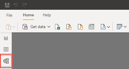
2. To link the two tables, go to the “Data Model” view of the report by clicking on the “data model” icon:

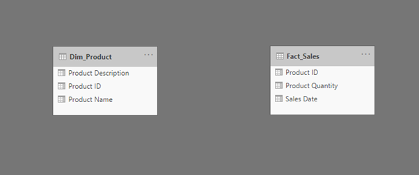
You should see the following tables:

Note: If Power BI has already created a relationship (showing a white arrow), you can right click the arrow and select “Delete” or “Properties” to work through the example from step 5.

3. To create the relationship, drag the “Product ID” field of one table and drop it onto the “Product ID” field of the other (see the diagram below):

This will automatically create a new relationship:

Editing Existing Relationships

To edit a relationship, right click on that white arrow and select “Properties”. This will open a new window:

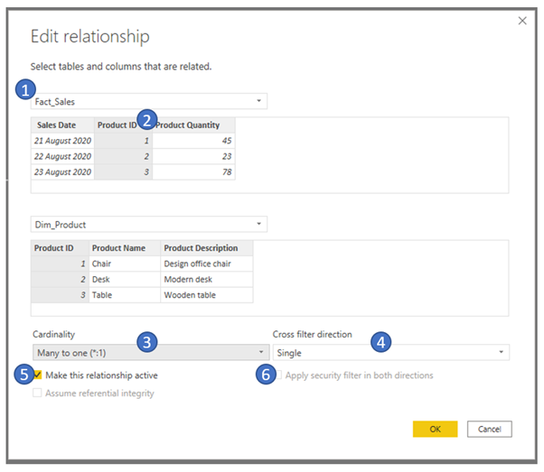
The “Edit relationship” window has several important components:

1. Using the dropdowns, you can select the tables to be linked by the relationship
2. By clicking on one of the columns shown in the table preview window, you can change the join key, i.e. the column that will link the two tables. In this example, the key is “Product ID” in both tables.
3. The cardinality can be chosen from the options described in the “Data Modelling Basics” section. The cardinality of the relationship studied in this example is many-to-one.
4. The cross-filter direction is a very important concept in Power BI data relationships. It determines how filters applied to a table will affect the other. If “Single” is selected here, filters applied to Dim_Product will also filter Fact_Sales. However, if “Both” is selected, filters applied to Fact_Sales will also filter Dim_Product. A good rule of thumb, especially as data models get more complex, is to use “Single” where possible, as this reduces the risk of circular data relationships (see the note at the end of this section). In most cases, filters are only applied from Dimension tables or Global filters.
5. In Power BI, relationship can be either “active” or “inactive”. Inactive relations cannot be used for visuals or filtering, and can be understood as “ghost” data relationships, visually represented as dashed arrows:

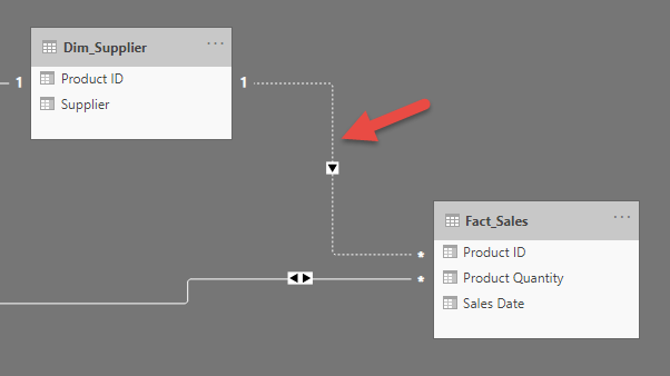
This type of relationships must only be used in very specific cases, when there is no need for joint visualisation or filtering, or when the USERELATIONSHIP DAX function can be used to change the nature of the relationship for certain calculations.

Here, the main rule of thumb is to use active relationships as much as possible, as inactive relationship cannot be used for cross-filtering and visuals.

Power BI sometimes greys out this “Make relationship active” checkbox. This is usually because an active relationship would generate circular data relationships (see the note at the end of this section). When this occurs, simply review the existing data model, trying to look for potential circular relationships. This problem is usually solved by changing the filtering directions from “Single” to “Both” where possible or removing relationships altogether.

6. Security filters are row-level security filters. As a quick reminder, in Power BI, developers can set security filters so that users only see the rows they are entitled to see. In this example, let’s say that the “Desk” Product Owner accesses the report, she should only view the data associated to “Desks”. This would be done by managing security roles in Power BI’s “Manage Roles” feature.

Security filters are very similar to regular filters, and just like regular filters, they could either be unidirectional or bidirectional. The example of the “Desk Product Owner” would only require a unidirectional security filters, as security flows from the Dim_Product to Fact_Sales, without the need to flow from Fact_Sales to Dim_Product. As a rule of thumb, it is a good idea to use single directional security filters as much as possible. This is partly because security filters, just like regular filters, can also create circular relationships…

Note on Circular Relationships

Circular data relationships occur when filters can flow in a circular manner between three or more table. The following example will illustrate this concept with the data table already used in the previous sections:

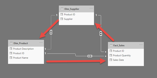
The relationship between Dim_Product and Dim_Supplier cannot be made active in this example, because it would create a circular relationship. This would mean that Dim_Product could filter Fact_Sales, that would then filter Dim_Supplier, that would in turn filter Dim_Product. This type of relationship is impossible, creating an infinite loop of filtering…

It is important to note that this is a very simple example, circular relationships could also occur with a very high number of tables. This highlights the need to keep data models as simple and deliberate as possible. These two ideas will be further explored in the following section.

Data Modelling Best Practices

As it has been stated above, the one-size-fits-all data model still has to be discovered. Despite this absence of optimal model, there exists several best practices to keep in mind when designing a Power BI data model.

1. Simplicity – Ockham’s Razor

Ockham’s razor might be one of the most quoted philosophical ideas in the world of analytics, and for a good reason! When it comes to data model, simple is usually good. The idea is to try to limit the number of tables and data relationships to a bare minimum.

2. Deliberateness

Even if simple is good, deliberate is better. “Deliberate” can be defined as “done with or marked by full consciousness of the nature and effects; intentional”. Each data modelling decision has to bear the final data visualisation objective in mind. Each table and data relationship must have a clearly defined purpose in the scope of the report being developed.

Wrapping Up

An efficient data model is the backbone of any enterprise Power BI reporting solution. This article’s main takeaway is that the optimal data model does not exist. Keeping the end visualisation goal and a few best practices in mind will already bring you a good part of the way there.

This article has been published from the source link without modifications to the text. Only the headline has been changed.

Source link