In this tutorial, you learn how to use Amazon SageMaker to build, train, and deploy a machine learning (ML) model using the XGBoost ML algorithm. Amazon SageMaker is a fully managed service that provides every developer and data scientist with the ability to build, train, and deploy machine learning (ML) models quickly.
Taking ML models from conceptualization to production is typically complex and time-consuming. You have to manage large amounts of data to train the model, choose the best algorithm for training it, manage the compute capacity while training it, and then deploy the model into a production environment. Amazon SageMaker reduces this complexity by making it much easier to build and deploy ML models. After you choose the right algorithms and frameworks from the wide range of choices available, SageMaker manages all of the underlying infrastructure to train your model at petabyte scale, and deploy it to production.
In this tutorial, you will assume the role of a machine learning developer working at a bank. You have been asked to develop a machine learning model to predict whether a customer will enroll for a certificate of deposit (CD).
In this tutorial, you learn how to:
- Create a SageMaker notebook instance
- Prepare the data
- Train the model to learn from the data
- Deploy the model
- Evaluate your ML model’s performance
The model will be trained on the Bank Marketing Data Set that contains information on customer demographics, responses to marketing events, and external factors. The data has been labeled for your convenience, and a column in the dataset identifies whether the customer is enrolled for a product offered by the bank. A version of this dataset is publicly available from the Machine Learning Repository curated by the University of California, Irvine.
The resources created and used in this tutorial are AWS Free Tier eligible. The cost of this workshop is less than $1.
Step 1. Create an Amazon SageMaker notebook instance for data preparation
In this step, you create the notebook instance that you use to download and process your data. As part of the creation process, you also create an Identity and Access Management (IAM) role that allows Amazon SageMaker to access data in Amazon S3.
a. Sign in to the Amazon SageMaker console, and in the top right corner, select your preferred AWS Region. This tutorial uses the US West (Oregon) Region.

b. In the left navigation pane, choose Notebook instances, then choose Create notebook instance.

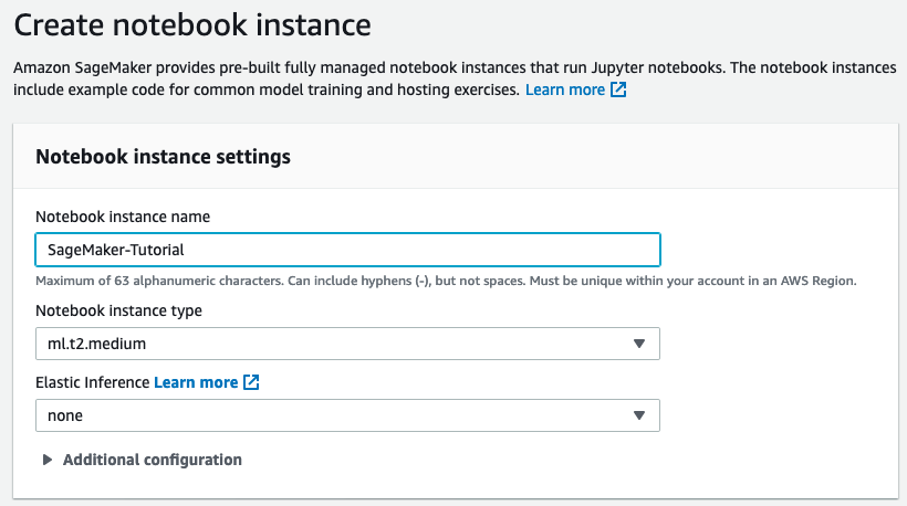
c. On the Create notebook instance page, in the Notebook instance setting box, fill the following fields:
- For Notebook instance name, type SageMaker-Tutorial.
- For Notebook instance type, choose ml.t2.medium.
- For Elastic inference, keep the default selection of none.
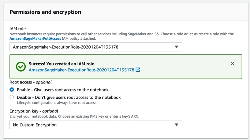
d. In the Permissions and encryption section, for IAM role, choose Create a new role, and in the Create an IAM role dialog box, select Any S3 bucket and choose Create role.
Note: If you already have a bucket that you’d like to use instead, choose Specific S3 buckets and specify the bucket name.
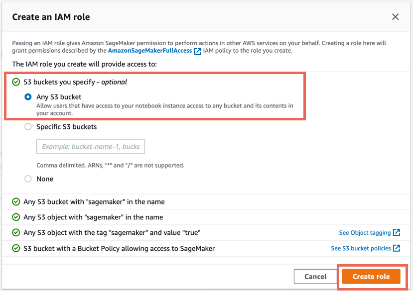
Amazon SageMaker creates the AmazonSageMaker-ExecutionRole-*** role.

Step 2. Prepare the data
In this step, you use your Amazon SageMaker notebook instance to preprocess the data that you need to train your machine learning model and then upload the data to Amazon S3.
a. After your SageMaker-Tutorial notebook instance status changes to InService, choose Open Jupyter.

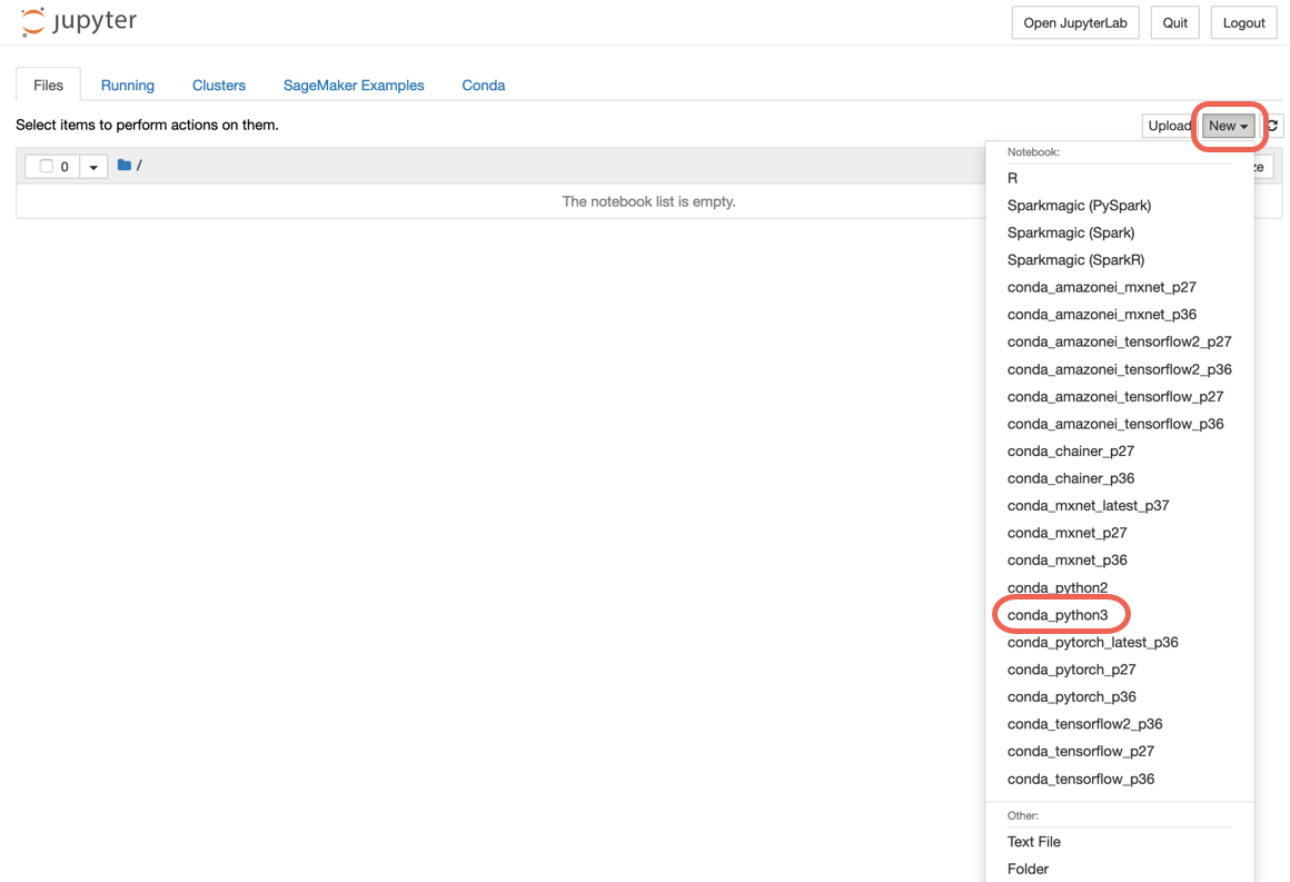
c. In a new code cell on your Jupyter notebook, copy and paste the following code and choose Run.
This code imports the required libraries and defines the environment variables you need to prepare the data, train the ML model, and deploy the ML model.
# import libraries
import boto3, re, sys, math, json, os, sagemaker, urllib.request
from sagemaker import get_execution_role
import numpy as np
import pandas as pd
import matplotlib.pyplot as plt
from IPython.display import Image
from IPython.display import display
from time import gmtime, strftime
from sagemaker.predictor import csv_serializer

# Define IAM role
role = get_execution_role()
prefix = 'sagemaker/DEMO-xgboost-dm'
my_region = boto3.session.Session().region_name # set the region of the instance

# this line automatically looks for the XGBoost image URI and builds an XGBoost container.
xgboost_container = sagemaker.image_uris.retrieve("xgboost", my_region, "latest")

print("Success - the MySageMakerInstance is in the " + my_region + "
d. Create the S3 bucket to store your data. Copy and paste the following code into the next code cell and choose Run.
Note: Make sure to replace the bucket_name your-s3-bucket-name with a unique S3 bucket name. If you don’t receive a success message after running the code, change the bucket name and try again.
bucket_name = 'your-s3-bucket-name' # <--- CHANGE THIS VARIABLE TO A UNIQUE NAME FOR YOUR BUCKET
s3 = boto3.resource('s3')
try:
    if  my_region == 'us-east-1':
      s3.create_bucket(Bucket=bucket_name)
    else:
      s3.create_bucket(Bucket=bucket_name, CreateBucketConfiguration={ 'LocationConstraint': my_region })
    print('S3 bucket created successfully')
except Exception as e:
    print('S3 error: ',e)
e. Download the data to your SageMaker instance and load the data into a dataframe. Copy and paste the following code into the next code cell and choose Run.
try:
  urllib.request.urlretrieve ("https://d1.awsstatic.com/tmt/build-train-deploy-machine-learning-model-sagemaker/bank_clean.27f01fbbdf43271788427f3682996ae29ceca05d.csv", "bank_clean.csv")
  print('Success: downloaded bank_clean.csv.')
except Exception as e:
  print('Data load error: ',e)

try:
  model_data = pd.read_csv('./bank_clean.csv',index_col=0)
  print('Success: Data loaded into dataframe.')
except Exception as e:
    print('Data load error: ',e)
f. Shuffle and split the data into training data and test data. Copy and paste the following code into the next code cell and choose Run.
The training data (70% of customers) is used during the model training loop. You use gradient-based optimization to iteratively refine the model parameters. Gradient-based optimization is a way to find model parameter values that minimize the model error, using the gradient of the model loss function.
The test data (remaining 30% of customers) is used to evaluate the performance of the model and measure how well the trained model generalizes to unseen data.
train_data, test_data = np.split(model_data.sample(frac=1, random_state=1729), [int(0.7 * len(model_data))])
print(train_data.shape, test_data.shape)
Step 3. Train the ML model
In this step, you use your training dataset to train your machine learning model.
a. In a new code cell on your Jupyter notebook, copy and paste the following code and choose Run.
This code reformats the header and first column of the training data and then loads the data from the S3 bucket. This step is required to use the Amazon SageMaker pre-built XGBoost algorithm.
pd.concat([train_data['y_yes'], train_data.drop(['y_no', 'y_yes'], axis=1)], axis=1).to_csv('train.csv', index=False, header=False)
boto3.Session().resource('s3').Bucket(bucket_name).Object(os.path.join(prefix, 'train/train.csv')).upload_file('train.csv')
s3_input_train = sagemaker.inputs.TrainingInput(s3_data='s3://{}/{}/train'.format(bucket_name, prefix), content_type='csv')
b. Set up the Amazon SageMaker session, create an instance of the XGBoost model (an estimator), and define the model’s hyperparameters. Copy and paste the following code into the next code cell and choose Run.
sess = sagemaker.Session()
xgb = sagemaker.estimator.Estimator(xgboost_container,role, instance_count=1, instance_type='ml.m4.xlarge',output_path='s3://{}/{}/output'.format(bucket_name, prefix),sagemaker_session=sess)
xgb.set_hyperparameters(max_depth=5,eta=0.2,gamma=4,min_child_weight=6,subsample=0.8,silent=0,objective='binary:logistic',num_round=100)
c. Start the training job. Copy and paste the following code into the next code cell and choose Run.
This code trains the model using gradient optimization on a ml.m4.xlarge instance. After a few minutes, you should see the training logs being generated in your Jupyter notebook.
xgb.fit({'train': s3_input_train})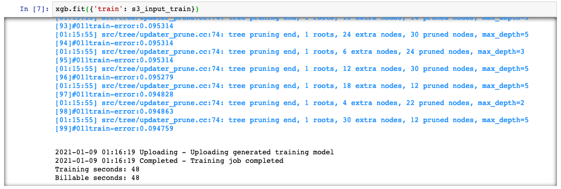
Step 4. Deploy the model
In this step, you deploy the trained model to an endpoint, reformat and load the CSV data, then run the model to create predictions.
a. In a new code cell on your Jupyter notebook, copy and paste the following code and choose Run.
This code deploys the model on a server and creates a SageMaker endpoint that you can access. This step may take a few minutes to complete.
xgb_predictor = xgb.deploy(initial_instance_count=1,instance_type='ml.m4.xlarge')
b. To predict whether customers in the test data enrolled for the bank product or not, copy the following code into the next code cell and choose Run.
from sagemaker.serializers import CSVSerializer

test_data_array = test_data.drop(['y_no', 'y_yes'], axis=1).values #load the data into an array
xgb_predictor.serializer = CSVSerializer() # set the serializer type
predictions = xgb_predictor.predict(test_data_array).decode('utf-8') # predict!
predictions_array = np.fromstring(predictions[1:], sep=',') # and turn the prediction into an array
print(predictions_array.shape)
Step 5. Evaluate model performance
In this step, you evaluate the performance and accuracy of the machine learning model.
In a new code cell on your Jupyter notebook, copy and paste the following code and choose Run.
This code compares the actual vs. predicted values in a table called a confusion matrix.
Based on the prediction, we can conclude that you predicted a customer will enroll for a certificate of deposit accurately for 90% of customers in the test data, with a precision of 65% (278/429) for enrolled and 90% (10,785/11,928) for didn’t enroll
cm = pd.crosstab(index=test_data['y_yes'], columns=np.round(predictions_array), rownames=['Observed'], colnames=['Predicted'])
tn = cm.iloc[0,0]; fn = cm.iloc[1,0]; tp = cm.iloc[1,1]; fp = cm.iloc[0,1]; p = (tp+tn)/(tp+tn+fp+fn)*100
print("\n{0:<20}{1:<4.1f}%\n".format("Overall Classification Rate: ", p))
print("{0:<15}{1:<15}{2:>8}".format("Predicted", "No Purchase", "Purchase"))
print("Observed")
print("{0:<15}{1:<2.0f}% ({2:<}){3:>6.0f}% ({4:<})".format("No Purchase", tn/(tn+fn)*100,tn, fp/(tp+fp)*100, fp))
print("{0:<16}{1:<1.0f}% ({2:<}){3:>7.0f}% ({4:<}) \n".format("Purchase", fn/(tn+fn)*100,fn, tp/(tp+fp)*100, tp))
Step 6. Clean up
In this step, you terminate the resources you used in this lab.
Important: Terminating resources that are not actively being used reduces costs and is a best practice. Not terminating your resources will result in charges to your account.
a. Delete your endpoint: In your Jupyter notebook, copy and paste the following code and choose Run.
xgb_predictor.delete_endpoint(delete_endpoint_config=True)b. Delete your training artifacts and S3 bucket: In your Jupyter notebook, copy and paste the following code and choose Run.
bucket_to_delete = boto3.resource('s3').Bucket(bucket_name)
bucket_to_delete.objects.all().delete()
c. Delete your SageMaker Notebook: Stop and delete your SageMaker Notebook.
- Open the SageMaker console.
- Under Notebooks, choose Notebook instances.
- Choose the notebook instance that you created for this tutorial, then choose Actions, Stop. The notebook instance takes up to several minutes to stop. When Status changes to Stopped, move on to the next step.
- Choose Actions, then Delete.
- Choose Delete.
This article has been published from the source link without modifications to the text. Only the headline has been changed.


