This article introduces everything you need in order to take off with BERT. We provide a step-by-step guide on how to fine-tune Bidirectional Encoder Representations from Transformers (BERT) for Natural Language Understanding and benchmark it with LSTM.
Motivation
Chatbots, virtual assistant, and dialog agents will typically classify queries into specific intents in order to generate the most coherent response. Intent classification is a classification problem that predicts the intent label for any given user query. It is usually a multi-class classification problem, where the query is assigned one unique label. For example, the query “how much does the limousine service cost within pittsburgh” is labeled as “groundfare” while the query “what kind of ground transportation is available in denver” is labeled as “ground_service”. The query “i want to fly from boston at 838 am and arrive in Denver at 1110 in the morning” is a “flight” intent, while “ show me the costs and times for flights from san francisco to atlanta” is an “airfare+flight_time” intent.
The examples above show how ambiguous intent labeling can be. Users might add misleading words, causing multiple intents to be present in the same query. Attention-based learning methods were proposed for intent classification (Liu and Lane, 2016; Goo et al., 2018). One type of network built with attention is called a Transformer. Itapplies attention mechanisms to gather information about the relevant context of a given word, and then encode that context in a rich vector that smartly represents the word.
In this article, we will demonstrate Transformer, especially how its attention mechanism helps in solving the intent classification task by learning contextual relationships. After demonstrating the limitation of a LSTM-based classifier, we introduce BERT: Pre-training of Deep Bidirectional Transformers, a novel Transformer-approach, pre-trained on large corpora and open-sourced. The last part of this article presents the Python code necessary for fine-tuning BERT for the task of Intent Classification and achieving state-of-art accuracy on unseen intent queries. We use the ATIS (Airline Travel Information System) dataset, a standard benchmark dataset widely used for recognizing the intent behind a customer query.
Intent classification with LSTM
Data
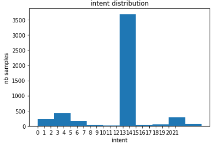
In one of our previous article, you will find the Python code for loading the ATIS dataset. In the ATIS training dataset, we have 26 distinct intents, whose distribution is shown below. The dataset is highly unbalanced, with most queries labeled as “flight” (code 14).
labels = intent_data_label_train
plt.hist(labels)
plt.xlabel('intent')
plt.ylabel('nb samples')
plt.title('intent distribution')
plt.xticks(np.arange(len(np.unique(labels))));
Multi-class classifier
Before looking at Transformer, we implement a simple LSTM recurrent network for solving the classification task. After the usual preprocessing, tokenization and vectorization, the 4978 samples are fed into a Keras Embedding layer, which projects each word as a Word2vec embedding of dimension 256. The results are passed through a LSTM layer with 1024 cells. This produces 1024 outputs which are given to a Dense layer with 26 nodes and softmax activation. The probabilities created at the end of this pipeline are compared to the original labels using categorical crossentropy.
model_lstm = Sequential()
model_lstm.add(Embedding(vocab_in_size, embedding_dim, input_length=len_input_train))
model_lstm.add(LSTM(units))
model_lstm.add(Dense(nb_labels, activation='softmax'))
model_lstm.compile(loss='categorical_crossentropy', optimizer='adam', metrics=['accuracy'])
model_lstm.summary()

history_lstm = model_lstm.fit(input_data_train, intent_data_label_cat_train,
                              epochs=10,batch_size=BATCH_SIZE)
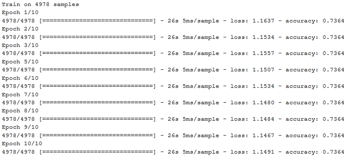
As we can see in the training output above, the Adam optimizer gets stuck, the loss and accuracy do not improve. The model appears to predict the majority class “flight” at each step.
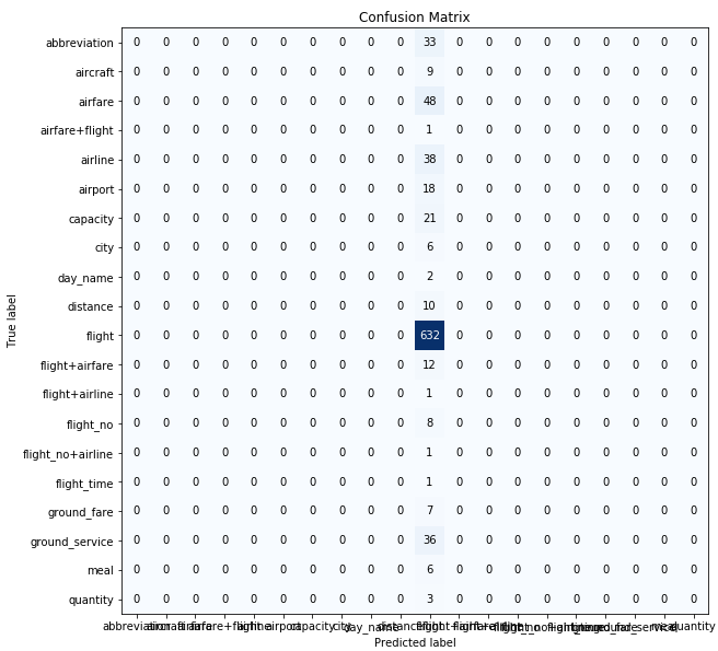
When we use the trained model to predict the intents on the unseen test dataset, the confusion matrix clearly shows how the model overfits to the majority “flight” class.
import scikitplot as skplt

def predict_intent(input_query, model=model_lstm, i2in=i2in_test, verbose=False):
  sv = query_to_vector(input_query)
  sv = sv.reshape(1,len(sv))
  intent_idx = np.argmax(model.predict(sv), axis=1)[0]
  intent_label = i2in[intent_idx]
  if verbose:
    print(intent_label)
  return intent_label, intent_idx

def evaluate_intent(queries, true_intents, model):
  predicted_intents = []
  for q in queries:
    intent_label, intent_idx = predict_intent(q, model)
    predicted_intents.append(intent_label)
  skplt.metrics.plot_confusion_matrix(true_intents, predicted_intents, figsize=(12,15))

true_intents = [i2in_test[i] for i in intent_data_label_test]
evaluate_intent(query_data_test, true_intents, model_lstm)
Data augmentation
Dealing with an imbalanced dataset is a common challenge when solving a classification task. Data augmentation is one thing that comes to mind as a good workaround. Here, it is not rare to encounter the SMOTE algorithm, as a popular choice for augmenting the dataset without biasing predictions. SMOTE uses a k-Nearest Neighbors classifier to create synthetic datapoints as a multi-dimensional interpolation of closely related groups of true data points. Unfortunately, we have 25 minority classes in the ATIS training dataset, leaving us with a single overly representative class. SMOTE fails to work as it cannot find enough neighbors (minimum is 2). Oversampling with replacement is an alternative to SMOTE, which also does not improve the model’s predictive performance either.
The SNIPS dataset, which is collected from the Snips personal voice assistant, a more recent dataset for natural language understanding, is a dataset which could be used to augment the ATIS dataset in a future effort.
Binary classifier
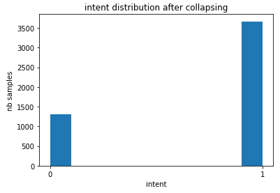
Since we were not quite successful at augmenting the dataset, now, we will rather reduce the scope of the problem. We define a binary classification task where the “flight” queries are evaluated against the remaining classes, by collapsing them into a single class called “other”. The distribution of labels in this new dataset is given below.
labels[labels==14] = -1
labels[labels!=-1] = 0
labels[labels==-1] = 1

plt.hist(labels)
plt.xlabel('intent')
plt.ylabel('nb samples')
plt.title('intent distribution after collapsing')
plt.xticks(np.arange(len(np.unique(labels))));
We can now use a similar network architecture as previously. The only change is to reduce the number of nodes in the Dense layer to 1, activation function to sigmoid and the loss function to binary crossentropy. Surprisingly, the LSTM model is still not able to learn to predict the intent, given the user query, as we see below.
model_lstm2 = Sequential()
model_lstm2.add(Embedding(vocab_in_size, embedding_dim, input_length=len_input_train))
model_lstm2.add(LSTM(units))
model_lstm2.add(Dense(1, activation='sigmoid'))
model_lstm2.compile(loss='binary_crossentropy', optimizer='adam', metrics=['accuracy'])

history_lstm2 = model_lstm2.fit(input_data_train, labels, epochs=10, batch_size=BATCH_SIZE)
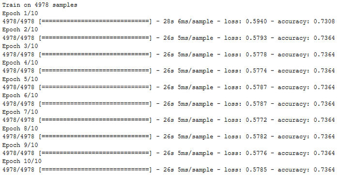
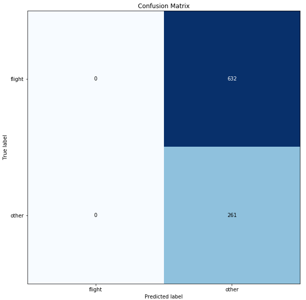
After 10 epochs, we evaluate the model on an unseen test dataset. This time, we have all samples being predicted as “other”, although “flight” had more than twice as many samples as “other” in the training set.
true_intents = ['flight' if i==14 else 'other' for i in intent_data_label_test]
predicted_intents = []
for q in query_data_test:
    intent_label, intent_idx = predict_intent(q, model_lstm2)
    predicted_intents.append('flight' if intent_idx==1 else 'other')

skplt.metrics.plot_confusion_matrix(true_intents, predicted_intents, figsize=(12,15))
Intent Classification with BERT
The motivation why we are now looking at Transformer is the poor classification result we witnessed with sequence-to-sequence models on the Intent Classification task when the dataset is imbalanced. In this section, we introduce a variant of Transformer and implement it for solving our classification problem. We will look especially at the late 2018 published Bidirectional Encoder Representations from Transformers (BERT).
What is BERT?
BERT is basically a trained Transformer Encoder stack, with twelve in the Base version, and twenty-four in the Large version, compared to 6 encoder layers in the original Transformer we described in the previous article.
BERT encoders have larger feedforward networks (768 and 1024 nodes in Base and Large respectively) and more attention heads (12 and 16 respectively). BERT was trained on Wikipedia and Book Corpus, a dataset containing +10,000 books of different genres. Below you can see a diagram of additional variants of BERT pre-trained on specialized corpora.
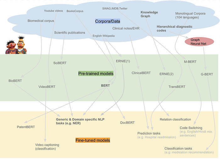
BERT was released to the public, as a new era in NLP. Its open-sourced model code broke several records for difficult language-based tasks. The pre-trained model on massive datasets enables anyone building natural language processing to use this free powerhouse. BERT theoretically allows us to smash multiple benchmarks with minimal task-specific fine-tuning.
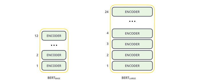
BERT works similarly to the Transformer encoder stack, by taking a sequence of words as input which keep flowing up the stack from one encoder to the next, while new sequences are coming in. The final output for each sequence is a vector of 728 numbers in Base or 1024 in Large version. We will use such vectors for our intent classification problem.
Why do we need BERT?
Proper language representation is key for general-purpose language understanding by machines. Context-free models such as word2vec or GloVe generate a single word embedding representation for each word in the vocabulary. For example, the word “bank” would have the same representation in “bank deposit” and in “riverbank”. Contextual models instead generate a representation of each word that is based on the other words in the sentence. BERT, as a contextual model, captures these relationships in a bidirectional way. BERT was built upon recent work and clever ideas in pre-training contextual representations including Semi-supervised Sequence Learning, Generative Pre-Training, ELMo, the OpenAI Transformer, ULMFit and the Transformer. Although these models are all unidirectional or shallowly bidirectional, BERT is fully bidirectional.
We will use BERT to extract high-quality language features from the ATIS query text data, and fine-tune BERT on a specific task (classification) with own data to produce state of the art predictions.
Preparing BERT environment
Feel free to download the original Jupyter Notebook, which we will adapt for our goal in this section.
As for development environment, we recommend Google Colab with its offer of free GPUs and TPUs, which can be added by going to the menu and selecting: Edit -> Notebook Settings -> Add accelerator (GPU). An alternative to Colab is to use a JupyterLab Notebook Instance on Google Cloud Platform, by selecting the menu AI Platform -> Notebooks -> New Instance -> Pytorch 1.1 -> With 1 NVIDIA Tesla K80 after requesting Google to increase your GPU quota. This will cost ca. $0.40 per hour (current pricing, which might change). Below you find the code for verifying your GPU availability.
# verify GPU availability
import tensorflow as tf

device_name = tf.test.gpu_device_name()
if device_name != '/device:GPU:0':
  raise SystemError('GPU device not found')
print('Found GPU at: {}'.format(device_name))
We will use the PyTorch interface for BERT by Hugging Face, which at the moment, is the most widely accepted and most powerful PyTorch interface for getting on rails with BERT. Hugging Face provides pytorch-transformers repository with additional libraries for interfacing more pre-trained models for natural language processing: GPT, GPT-2, Transformer-XL, XLNet, XLM.
As you can see below, in order for torch to use the GPU, you have to identify and specify the GPU as the device, because later in the training loop, we load data onto that device.
# install
!pip install pytorch-pretrained-bert pytorch-nlp

# BERT imports
import torch
from torch.utils.data import TensorDataset, DataLoader, RandomSampler, SequentialSampler
from keras.preprocessing.sequence import pad_sequences
from sklearn.model_selection import train_test_split
from pytorch_pretrained_bert import BertTokenizer, BertConfig
from pytorch_pretrained_bert import BertAdam, BertForSequenceClassification
from tqdm import tqdm, trange
import pandas as pd
import io
import numpy as np
import matplotlib.pyplot as plt
% matplotlib inline

# specify GPU device
device = torch.device("cuda" if torch.cuda.is_available() else "cpu")
n_gpu = torch.cuda.device_count()
torch.cuda.get_device_name(0)
Now we can upload our dataset to the notebook instance. Please run the code from our previous article to preprocess the dataset using the Python function load_atis() before moving on.
BERT expects input data in a specific format, with special tokens to mark the beginning ([CLS]) and separation/end of sentences ([SEP]). Furthermore, we need to tokenize our text into tokens that correspond to BERT’s vocabulary.
'[CLS]  i want to fly from boston at 838 am and arrive in denver at 1110 in the morning  [SEP]'

['[CLS]', 'i', 'want', 'to', 'fly', 'from', 'boston', 'at', '83', '##8', 'am', 'and', 'arrive', 'in', 'denver', 'at', '111', '##0', 'in', 'the', 'morning', '[SEP]']
For each tokenized sentence, BERT requires input ids, a sequence of integers identifying each input token to its index number in the BERT tokenizer vocabulary.
# Set the maximum sequence length.
MAX_LEN = 128
# Pad our input tokens
input_ids = pad_sequences([tokenizer.convert_tokens_to_ids(txt) for txt in tokenized_texts],
                          maxlen=MAX_LEN, dtype="long", truncating="post", padding="post")
# Use the BERT tokenizer to convert the tokens to their index numbers in the BERT vocabulary
input_ids = [tokenizer.convert_tokens_to_ids(x) for x in tokenized_texts]
input_ids = pad_sequences(input_ids, maxlen=MAX_LEN, dtype="long", truncating="post", padding="post")
BERT’s clever language modeling task masks 15% of words in the input and asks the model to predict the missing word. To make BERT better at handling relationships between multiple sentences, the pre-training process also included an additional task: given two sentences (A and B), is B likely to be the sentence that follows A? Therefore we need to tell BERT what task we are solving by using the concept of attention mask and segment mask. In our case, all words in a query will be predicted and we do not have multiple sentences per query. We define the mask below.
# Create attention masks
attention_masks = []
# Create a mask of 1s for each token followed by 0s for padding
for seq in input_ids:
  seq_mask = [float(i>0) for i in seq]
  attention_masks.append(seq_mask)
Now it is time to create all tensors and iterators needed during fine-tuning of BERT using our data.
# Use train_test_split to split our data into train and validation sets for training
train_inputs, validation_inputs, train_labels, validation_labels = train_test_split(input_ids, labels,
                                                            random_state=2018, test_size=0.1)
train_masks, validation_masks, _, _ = train_test_split(attention_masks, input_ids,
                                             random_state=2018, test_size=0.1)

# Convert all of our data into torch tensors, the required datatype for our model
train_inputs = torch.tensor(train_inputs)
validation_inputs = torch.tensor(validation_inputs)
train_labels = torch.tensor(train_labels)
validation_labels = torch.tensor(validation_labels)
train_masks = torch.tensor(train_masks)
validation_masks = torch.tensor(validation_masks)

# Select a batch size for training.
batch_size = 32

# Create an iterator of our data with torch DataLoader
train_data = TensorDataset(train_inputs, train_masks, train_labels)
train_sampler = RandomSampler(train_data)
train_dataloader = DataLoader(train_data, sampler=train_sampler, batch_size=batch_size)
validation_data = TensorDataset(validation_inputs, validation_masks, validation_labels)
validation_sampler = SequentialSampler(validation_data)
validation_dataloader = DataLoader(validation_data, sampler=validation_sampler, batch_size=batch_size)
Finally, it is time to fine-tune the BERT model so that it outputs the intent class given a user query string. For this purpose, we use the BertForSequenceClassification, which is the normal BERT model with an added single linear layer on top for classification. Below we display a summary of the model. The encoder summary is shown only once. The same summary would normally be repeated 12 times. We display only 1 of them for simplicity sake. We can see the BertEmbedding layer at the beginning, followed by a Transformer architecture for each encoder layer: BertAttention, BertIntermediate, BertOutput. At the end, we have the Classifier layer.
# Load BertForSequenceClassification, the pretrained BERT model with a single linear classification layer on top.

model = BertForSequenceClassification.from_pretrained("bert-base-uncased", num_labels=nb_labels)
model.cuda()

# BERT model summary
BertForSequenceClassification(
  (bert): BertModel(
    (embeddings): BertEmbeddings(
      (word_embeddings): Embedding(30522, 768, padding_idx=0)
      (position_embeddings): Embedding(512, 768)
      (token_type_embeddings): Embedding(2, 768)
      (LayerNorm): BertLayerNorm()
      (dropout): Dropout(p=0.1)
    )
    (encoder): BertEncoder(
      (layer): ModuleList(
        (0): BertLayer(
          (attention): BertAttention(
            (self): BertSelfAttention(
              (query): Linear(in_features=768, out_features=768, bias=True)
              (key): Linear(in_features=768, out_features=768, bias=True)
              (value): Linear(in_features=768, out_features=768, bias=True)
              (dropout): Dropout(p=0.1)
            )
            (output): BertSelfOutput(
              (dense): Linear(in_features=768, out_features=768, bias=True)
              (LayerNorm): BertLayerNorm()
              (dropout): Dropout(p=0.1)
            )
          )
          (intermediate): BertIntermediate(
            (dense): Linear(in_features=768, out_features=3072, bias=True)
          )
          (output): BertOutput(
            (dense): Linear(in_features=3072, out_features=768, bias=True)
            (LayerNorm): BertLayerNorm()
            (dropout): Dropout(p=0.1)
          )
        )
        '
        '
        '
      )
    )
    (pooler): BertPooler(
      (dense): Linear(in_features=768, out_features=768, bias=True)
      (activation): Tanh()
    )
  )
  (dropout): Dropout(p=0.1)
  (classifier): Linear(in_features=768, out_features=2, bias=True)
)
As we feed input data, the entire pre-trained BERT model and the additional untrained classification layer is trained on our specific task. Training the classifier is relatively inexpensive. The bottom layers have already great English words representation, and we only really need to train the top layer, with a bit of tweaking going on in the lower levels to accommodate our task. This is a variant of transfer learning.
# BERT fine-tuning parameters
param_optimizer = list(model.named_parameters())
no_decay = ['bias', 'gamma', 'beta']
optimizer_grouped_parameters = [
    {'params': [p for n, p in param_optimizer if not any(nd in n for nd in no_decay)],
     'weight_decay_rate': 0.01},
    {'params': [p for n, p in param_optimizer if any(nd in n for nd in no_decay)],
     'weight_decay_rate': 0.0}
]

optimizer = BertAdam(optimizer_grouped_parameters,
                     lr=2e-5,
                     warmup=.1)

# Function to calculate the accuracy of our predictions vs labels
def flat_accuracy(preds, labels):
    pred_flat = np.argmax(preds, axis=1).flatten()
    labels_flat = labels.flatten()
    return np.sum(pred_flat == labels_flat) / len(labels_flat)

# Store our loss and accuracy for plotting
train_loss_set = []
# Number of training epochs
epochs = 4

# BERT training loop
for _ in trange(epochs, desc="Epoch"):

  ## TRAINING

  # Set our model to training mode
  model.train()
  # Tracking variables
  tr_loss = 0
  nb_tr_examples, nb_tr_steps = 0, 0
  # Train the data for one epoch
  for step, batch in enumerate(train_dataloader):
    # Add batch to GPU
    batch = tuple(t.to(device) for t in batch)
    # Unpack the inputs from our dataloader
    b_input_ids, b_input_mask, b_labels = batch
    # Clear out the gradients (by default they accumulate)
    optimizer.zero_grad()
    # Forward pass
    loss = model(b_input_ids, token_type_ids=None, attention_mask=b_input_mask, labels=b_labels)
    train_loss_set.append(loss.item())
    # Backward pass
    loss.backward()
    # Update parameters and take a step using the computed gradient
    optimizer.step()
    # Update tracking variables
    tr_loss += loss.item()
    nb_tr_examples += b_input_ids.size(0)
    nb_tr_steps += 1
  print("Train loss: {}".format(tr_loss/nb_tr_steps))

  ## VALIDATION

  # Put model in evaluation mode
  model.eval()
  # Tracking variables
  eval_loss, eval_accuracy = 0, 0
  nb_eval_steps, nb_eval_examples = 0, 0
  # Evaluate data for one epoch
  for batch in validation_dataloader:
    # Add batch to GPU
    batch = tuple(t.to(device) for t in batch)
    # Unpack the inputs from our dataloader
    b_input_ids, b_input_mask, b_labels = batch
    # Telling the model not to compute or store gradients, saving memory and speeding up validation
    with torch.no_grad():
      # Forward pass, calculate logit predictions
      logits = model(b_input_ids, token_type_ids=None, attention_mask=b_input_mask)
    # Move logits and labels to CPU
    logits = logits.detach().cpu().numpy()
    label_ids = b_labels.to('cpu').numpy()
    tmp_eval_accuracy = flat_accuracy(logits, label_ids)
    eval_accuracy += tmp_eval_accuracy
    nb_eval_steps += 1
  print("Validation Accuracy: {}".format(eval_accuracy/nb_eval_steps))

# plot training performance
plt.figure(figsize=(15,8))
plt.title("Training loss")
plt.xlabel("Batch")
plt.ylabel("Loss")
plt.plot(train_loss_set)
plt.show()

The training loss plot from the variable train_loss_set looks awesome. The whole training loop took less than 10 minutes.
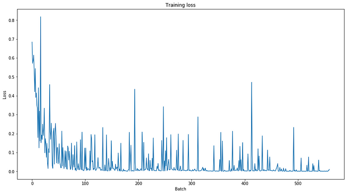
Now, it is the moment of truth. Is BERT overfitting? Or is it doing better than our previous LSTM network? We now load the test dataset and prepare inputs just as we did with the training set. We then create tensors and run the model on the dataset in evaluation mode.
# load test data
sentences = ["[CLS] " + query + " [SEP]" for query in query_data_test]
labels = intent_data_label_test

# tokenize test data
tokenized_texts = [tokenizer.tokenize(sent) for sent in sentences]
MAX_LEN = 128
# Pad our input tokens
input_ids = pad_sequences([tokenizer.convert_tokens_to_ids(txt) for txt in tokenized_texts],
                          maxlen=MAX_LEN, dtype="long", truncating="post", padding="post")
# Use the BERT tokenizer to convert the tokens to their index numbers in the BERT vocabulary
input_ids = [tokenizer.convert_tokens_to_ids(x) for x in tokenized_texts]
input_ids = pad_sequences(input_ids, maxlen=MAX_LEN, dtype="long", truncating="post", padding="post")
# Create attention masks
attention_masks = []
# Create a mask of 1s for each token followed by 0s for padding
for seq in input_ids:
  seq_mask = [float(i>0) for i in seq]
  attention_masks.append(seq_mask)

# create test tensors
prediction_inputs = torch.tensor(input_ids)
prediction_masks = torch.tensor(attention_masks)
prediction_labels = torch.tensor(labels)
batch_size = 32
prediction_data = TensorDataset(prediction_inputs, prediction_masks, prediction_labels)
prediction_sampler = SequentialSampler(prediction_data)
prediction_dataloader = DataLoader(prediction_data, sampler=prediction_sampler, batch_size=batch_size)

## Prediction on test set
# Put model in evaluation mode
model.eval()
# Tracking variables
predictions , true_labels = [], []
# Predict
for batch in prediction_dataloader:
  # Add batch to GPU
  batch = tuple(t.to(device) for t in batch)
  # Unpack the inputs from our dataloader
  b_input_ids, b_input_mask, b_labels = batch
  # Telling the model not to compute or store gradients, saving memory and speeding up prediction
  with torch.no_grad():
    # Forward pass, calculate logit predictions
    logits = model(b_input_ids, token_type_ids=None, attention_mask=b_input_mask)
  # Move logits and labels to CPU
  logits = logits.detach().cpu().numpy()
  label_ids = b_labels.to('cpu').numpy()
  # Store predictions and true labels
  predictions.append(logits)
  true_labels.append(label_ids)

# Import and evaluate each test batch using Matthew's correlation coefficient
from sklearn.metrics import matthews_corrcoef
matthews_set = []
for i in range(len(true_labels)):
  matthews = matthews_corrcoef(true_labels[i],
                 np.argmax(predictions[i], axis=1).flatten())
  matthews_set.append(matthews)

# Flatten the predictions and true values for aggregate Matthew's evaluation on the whole dataset
flat_predictions = [item for sublist in predictions for item in sublist]
flat_predictions = np.argmax(flat_predictions, axis=1).flatten()
flat_true_labels = [item for sublist in true_labels for item in sublist]

print('Classification accuracy using BERT Fine Tuning: {0:0.2%}'.format(matthews_corrcoef(flat_true_labels, flat_predictions)))
With BERT we are able to get a good score (95.93%) on the intent classification task. This demonstrates that with a pre-trained BERT model it is possible to quickly and effectively create a high-quality model with minimal effort and training time using the PyTorch interface.
Conclusion
In this article, I demonstrated how to load the pre-trained BERT model in a PyTorch notebook and fine-tune it on your own dataset for solving a specific task. Attention matters when dealing with natural language understanding tasks. When combined with powerful words embedding from Transformer, an intent classifier can significantly improve its performance, as we successfully exposed.
My new article provides hands-on proven PyTorch code for question answering with BERT fine-tuned on the SQuAD dataset.


