How does Deep Learning apply to Unsupervised Learning? An intuitive introduction to Autoencoders!
Machine Learning is often classified into three categories:
- Supervised Learning
- Unsupervised Learning
- Reinforcement Learning (will be covered in Part 4 of the introductory series)
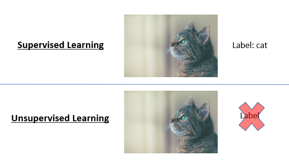
The difference between these categories largely lies in the type of data that we are dealing with: Supervised Learning deals with labelled data (the label is the ‘true value’ of the thing we are trying to predict), while Unsupervised Learning deals with unlabeled data.
To illustrate the distinctions between supervised and unsupervised learning, take the example of images. Supervised Learning deals with the case where we have the images and the labels of what is contained in the image (e.g. cat). Unsupervised Learning deals with the case where we just have the images.

Given the labels of images in our training dataset, we can find the patterns of how the pixel values translate to what’s inside our image. For example, we can use a Convolutional Neural Networks (Part 2 of our introductory series) to do that pattern recognition from the data we have. Without the labels, however, we can only often find patterns and structure within the data. There is no way to recognize whether there is a cat in the image if you’ve never told the model what a cat even looks like!
A good example of Unsupervised Learning is clustering, where we find clusters within the data set based on the underlying data itself. The field of Unsupervised Learning is still currently rather under-developed in my opinion, which is a pity because we have a whole ton of unlabeled data out there. After all, many of the images that we have (such as the photographs that we take) are not nicely labelled!
Thus far, we’ve always assumed that we have the labels to train our neural networks. As a recap of why we need labels in training our neural network: the label tells us whether the model’s prediction is correct or not, and this contributes to our loss function which we can minimize by changing the parameters using stochastic gradient descent. While it’s not entirely obvious how neural networks might apply to Unsupervised Learning, I hope that by the end of this post you’ll see how clever engineering can use neural networks for Unsupervised Learning.
Summary: Unsupervised Learning deals with data without labels.
The problem we wish to tackle with auto-encoders is: Given that the data that has many features, can we construct a smaller set of features to represent the information in the data? As a very simplistic example, suppose I have a dataset of persons and I know these two features about them:
- Color of eyes: whether their eyes are blue or black (0 for blue, 1 for black)
- Gender: whether they are male or female (0 for male, 1 for female)
This corresponds to two input features. But is there a way to represent our data with less features?
What if we had a neuron that took in those two features and transformed it like this:

The possible combinations of color of eyes and gender will be represented by the neuron like this:

Notice that we’ve reduced our feature set to only have one feature (which we call ‘neuron’ here) instead of our original two. Nevertheless, we have still represented the input features well. It should be obvious that we haven’t really lost any information from the data, and so we’ve found a more condensed representation for our data. This is called dimensionality reduction.
How do we know whether the data is well-represented by our neuron, or whether some information has been lost along the way? Simple. The test is this: How well can we reconstruct the neuron back into its original two features?
Suppose we have some function, represented by the arrow in green, that takes the neuron value and reconstructs it back to the original two features:

Since the reconstructed features exactly match the original features, it means we haven’t lost any information at all in our neuron. The blue arrow above has done its job perfectly in finding a compressed representation that preserves the original data; and the green arrow has done its job perfectly in reconstructing the data!
Summary: An example of Unsupervised Learning is dimensionality reduction, where we condense the data into fewer features while retaining as much information as possible.
Thus far, we’ve covered a very simplistic example; however, auto-encoders in practice are not far off in intuition. Recall that the blue and green arrows are simply functions that convert a large set of features into a smaller set of features and vice versa. Since neural networks are essentially complicated functions (recall Part 1a), we can use neural networks as the blue and green arrows! And that, in essence, is an auto-encoder!

Just for terminology sake, we call the blue arrow the encoder and the green arrow the decoder. The smaller set of features that represent the data is called the encoding.
Now that we understand what the auto-encoder is trying to do, how do we train it? After all, we said at the start that labels are required to train our neural network! For this, we require some clever engineering based on some astute observations.
The first thing that we might have tried to do is to try to train the encoder and decoder as separate neural networks. However, we soon face the problem that we do not know the ground truth of what the encoding (compressed set of features) ought to be. There is no label to say that the input features should correspond to this particular encoding. Thus, it’s impossible to train our encoder! Without the encoder, we will not have the encoding and thus we have no input features to the decoder! This makes it impossible to train our decoder as well!

You might be wondering why I say that the decoder has labels in the table above. Where did these labels come from? After all, we do not have any external labels.
We must ask ourselves: What is the objective of the decoder? What is the ‘ground truth’ value that we are trying to output?
Let’s take an example. Suppose we wish to encode an image of a cat into some compressed set of features. The point of the decoder is to reconstruct the image of the cat. What is the ‘ground truth’ label for the decoder? The original image of the cat!

Ok, so we have a label for the decoder. But that doesn’t solve our initial problem: we don’t have the label for the encoder and the input for the decoder.
To address this problem, we train the encoder and decoder as one large neural network rather than separately. The input features for our encoder is the input features for our large neural network. The label for our decoder is the label for our large neural network. This way, we have both the input features and label necessary to train our neural network:

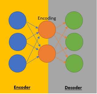
It is not by accident that I called the encoding a “neuron” in the simplistic example I gave earlier. The output of the encoder is a set of neurons that forms the encoding (compressed set of features). The input of the decoder is the very same set of neurons in the encoding (compressed set of features). Since the input of a layer in the neural network is the output of the neurons in the previous layer, we can combine the encoder and decoder into a giant neural network like this:

Notice that while the encoder is on the left side and the decoder is on the right side, together they form one big neural network with three layers (blue, orange and green).
Of course, auto-encoders in practice have more layers in the encoder and decoder. In fact, they don’t even have to be fully-connected layers like we’ve shown above. Most image auto-encoders will have convolutional layers, and other layers we’ve seen in neural networks. The one thing they must have, however, is a bottleneck layer that corresponds to the encoding.
The point of the auto-encoder is to reduce the feature dimensions. If, in the above diagram, we had four orange neurons instead of two, then our encoding has more features than the input! This totally defeats the purpose of auto-encoders in the first place.
So now that we’ve got our large neural network architecture, how do we train it? Recall that the label of the decoder is now the label of this large neural network, and the label of the decoder was our original input data. Therefore, the label for our large neural network is exactly the same as the original input data to this large neural network!
For us to apply our neural networks and whatever we’ve learnt in Part 1a, we need to have a loss function that tells us how we are doing. We then find the best parameters that minimizes the loss function. This much has not changed. In other tasks, the loss function comes from how far away our output neuron is from the ground truth value. In this task, the loss function comes from how far away our output neuron is from our input neuron!
Given that the task is to encode and reconstruct, this makes intuitive sense. If the output neurons match the original data points perfectly, this means that we have successfully reconstructed the input. Since the neural network has a bottleneck layer, it must then mean that the fewer set of features in the encoding contains all the data it needs, which means we have a perfect encoder. This is the gold standard. Now, the auto-encoder may not be perfect, but the closer we can get to this gold standard, the better.
In essence, training an auto-encoder means:
- Training a neural network with a ‘bottleneck layer’ within our neural network. The bottleneck layer has less features than the input layer. Everything to the left of the bottleneck layer is the encoder; everything to the right is the decoder.
- The label that we compare our output against is the input to the neural network. Since we now have a label, we can apply our standard neural network training that we’ve learnt in Part 1a and Part 1b as though this was a Supervised Learning task.
And there we have it, our auto-encoder!
Summary: An auto-encoder uses a neural network for dimensionality reduction. This neural network has a bottleneck layer, which corresponds to the compressed vector. When we train this neural network, the ‘label’ of our output is our original input. Thus, the loss function we minimize corresponds to how poorly the original data is reconstructed from the compressed vector.
Consolidated Summary: Unsupervised Learning deals with data without labels. An example of Unsupervised Learning is dimensionality reduction, where we condense the data into fewer features while retaining as much information as possible. An auto-encoder uses a neural network for dimensionality reduction. This neural network has a bottleneck layer, which corresponds to the compressed vector. When we train this neural network, the ‘label’ of our output is our original input. Thus, the loss function we minimize corresponds to how poorly the original data is reconstructed from the compressed vector.
What’s Next: We’ve gone through a brief overview on the vanilla auto-encoder, which is useful for dimensionality reduction, i.e. encoding data into a more compressed representation with less features. This is useful for applications such as visualizing on fewer axes or reducing the feature set size before passing it through another neural network.
In a future post, we will go through a popular and more advanced variant of the auto-encoder, called variational autoencoders (VAEs). VAEs are used for applications such as image generation. A simple VAE, for example, is able to generate the faces of fictional celebrities like this:

You’ll need the concepts in this post as a pre-requisite, so don’t forget what you’ve learnt here today! Till next time!
This article has been published from the source link without modifications to the text. Only the headline has been changed.


