A non-convoluted look into graph theory and machine learning
In my last article on graph theory, I briefly introduced my latest topic of interest: Graph Convolutional Networks. If you’re here thinking “what do those words mean?”, you’re in the right place. In this article, we’re going to break this topic down, step by step.
Part I: What’s This Graph Thing?
If this is the first you’re hearing this ‘graph’ word, I’m sorry, but you have some homework to do. Before we can dive deeper into this topic, you should check out my last article briefly introducing graph theory (and why we care about it). I’ll wait here!
Alright, now that you’re back, let’s explain a bit further. Graph theory is a mathematical theory, which simply defines a graph as:
G = (v, e) where G is our graph, and (v, e) represents a set of vertices or nodes as computer scientists tend to call them, and edges, or connections between these nodes. Graph theory exists because we need a way computationally and mathematically to represent relationships between things.These things can be anything: users on a social media platform, physical neighbors in a community, addresses or locations (coordinates) on a map, pixels in an image, or neurons in our brain. The basis of graph theory as it relates to machine learning in particular is that much of our data can be best understood when we can represent its relationships. Therefore, we’d like a way to embed these relationships so that we can then work with the whole of the data.
But let’s not get too far ahead of ourselves — we have some more terms to define.
Part II: Convolution? That sounds… convoluted.
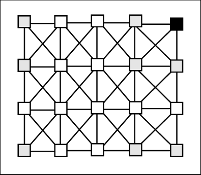
Let’s bring it back to the things which have relationships with other things that we want to understand. Simple enough, right? Let’s consider, for example, we have pixels in an image. Those pixels are always related to every other pixel in an image. This image has a set structure, and the pixels remain within proximity to other pixels in a fixed way. Let’s take a look:

If you can tell, this fits our definition of a graph. Implicitly, an image is ‘viewed’ as a graph by a different type of neural network: a Convolutional Neural Network. In this article, I’ll be breezing through the very basic concepts of convolutional neural networks to explain graph convolutional nets. However, if you aren’t aware of CNN’s, I highly recommend taking a look at the linked source after reading this article to gain a well-rounded understanding of all of these topics.
You may be able to intuit from their name that graph convolutional networks and convolutional neural networks share some things in common. You would be correct to think this — the intuition behind GCN’s and CNN’s is extraordinarily similar.
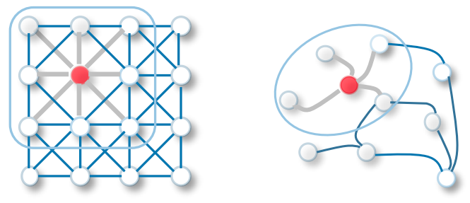
But what is our CNN doing with this image above? If it’s technically a graph, why do we need this other thing? Well, I’m glad you asked!
Images are implicitly graphs of pixels connected to other pixels, but they always have a fixed structure. As our convolutional neural network is sharing weights across neighboring cells, it does so based on some assumptions: for example, that we can evaluate a 3 x 3 area of pixels as a “neighborhood”. The assumptions on which our convolutional neural networks work rely on 2-dimensonal, regular data (also called Euclidean data, if you’re well-versed in domain terminology).
Our social media networks, molecular structure representations, or addresses on a map aren’t two-dimensional, though. They also don’t have a necessary size or structure. We encounter difficulty when trying to cram non-Euclidean or arbitrarily structured data into CNN’s, since that’s about where they reach their limit and stop being useful.
Part III: Networks

We’ve established that we have these arbitrarily structured networks of stuff that don’t fit into our traditional convolutional neural networks. In fact, they don’t really work with a lot of different kinds of neural networks. As such, there are graph neural networks, of which graph convolutional networks are a basic variant.
In this article, I won’t be getting into the mathematics behind graph convolutional networks (even though it’s quite fun) — I just want to discuss the intuition. (Don’t worry — I cover the mathematics in the next article of the series.)
Effectively, the primary difficulty in embedding features represented as both nodes and edges is this matter of arbitrary space usage, and a lack of Euclidean distance between neighbors. With those facets, we must base approaches off of different assumptions. Here, I’ll be primarily discussing graph convolutional networks as they’ve been discussed by Kipf & Welling, although there are various approaches.
We’ve learned about how convolution in neural networks is a method of sharing weights between neighbors. First, to determine neighbors, we’re going to need to provide some data.
Where the normal neural network forward propagation function determines the feature representation of the next hidden layer by evaluating our weights, feature representation and bias for our current layer, our graph convolutional network is going to add an adjacency matrix to the equation. There is also our non-linear activation function, which, since I’m trying to not get too mathematical, I’m ignoring in our considerations for now.
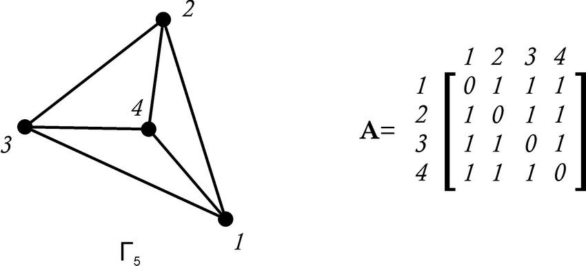
Do we remember what an adjacency matrix looks like? Here’s a refresher:

What A is is a matrix representation of the connections within our graph, ????₅. Each row or column label represents the node with the same number label, and a 1 in an intersecting row/column represents an edge between those nodes.
For those of you familiar with machine learning already, this looks a bit like a sparse matrix, right? See, this isn’t all so new after all.
Effectively, representing our graph as an adjacency matrix enables us to provide it to the net in the form of a tensor, something our model can work with.
Before we can just hand this matrix over to our propagation equation, though, we need to ensure that we normalize our values. The intuition behind this is similar to normalizing any data we feed through a neural network: values of vastly different degrees of magnitude can cause our network to learn higher weights for values that it shouldn’t, simply because those values were initially much higher than other values. For our purposes here, we’re just going to mention normalization. I’ll dive more deeply into Kipf & Welling’s methodology and intuition in the next article.
Once we’ve normalized our data, we’ll perform some kind of aggregation between neighboring nodes — for example, take an average. The intuition here for semi-supervised learning is that similar nodes are likely to share the same label. We can imagine this process as the passing of a message, where each layer of our GCN takes an aggregate of a neighbor node, and passes it one “hop” away, to the next node.
So if we have a three-layer GCN, we can convolve each node’s ‘third-order’ neighborhood. In human terms, this means that we can pass a message to each node’s neighbor three “hops” away and effectively embed the community structure of our graph. If, however, we have a graph with many more “hops”, we would need more layers to effectively embed our graph structure.
If you’re feeling anything like I did when I first delved into this topic, you’re probably ready for a break. Before I let you off the hook, let’s take a look at what we’ve learned:
- We’ve recapped the essentials of graph theory, and understood why we care about this as machine learning engineers and data scientists.
- We’ve looked at convolutional neural networks, evaluated the term “convolution” briefly, and discussed their limitations.
- We’ve taken a brief peek behind the scenes of the intuition behind graph convolutional networks, and we mostly understand why they work!
Alright, take a rest for now, and don’t forget to give yourself a pat on the back! You’ve learned a lot in a short span. I look forward to next time, where we’ll dive deeper into the mathematics that make all of this work, and learn how to start coding up our very own GCN.
Source link


